The Harmonic Oscillator
Posted 11th February 2022 by Holger Schmitz
I wasn’t really planning on writing this post. I was preparing a different post when I found that I needed to explain a property of the so-called “harmonic oscillator”. I first thought about adding a little excursion into the article that I was going to write. But I found that the harmonic oscillator is such an important concept in physics that it would not be fair to deny it its own post. The harmonic oscillator appears in many contexts and I don’t think there is any branch in physics that can do without it.
The Spring-and-Mass System
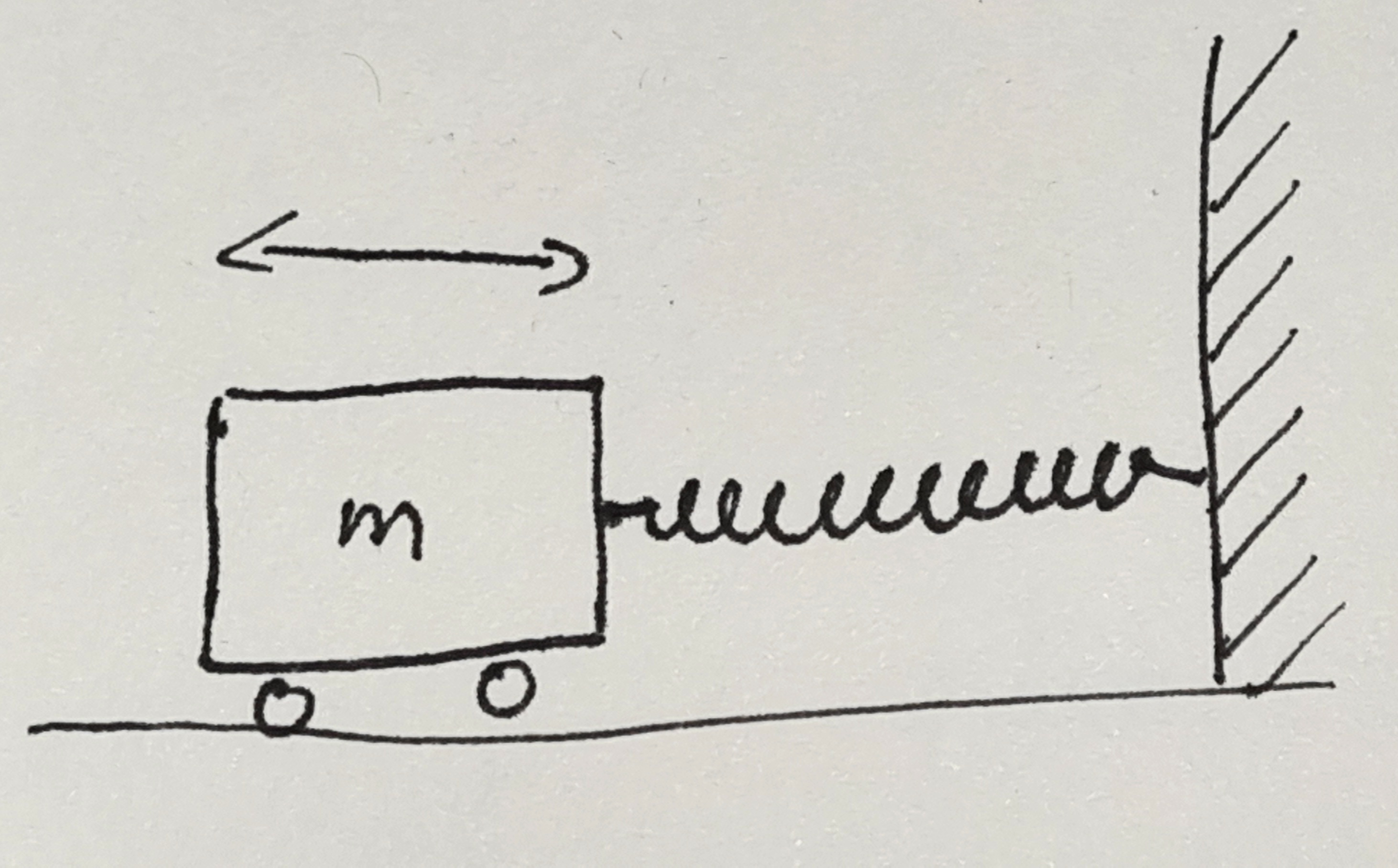
Let’s start with the most simple system that you will probably know from school. The mass on a spring is an idealized system consisting of a mass \(m\) attached to one end of a spring. The other end of the spring is held fixed. We imagine it being attached to a strong wall that will not move. The mass can only move in one direction and this motion will act to extend or contract the spring. The spring itself is assumed to be very light so that we can ignore its mass.
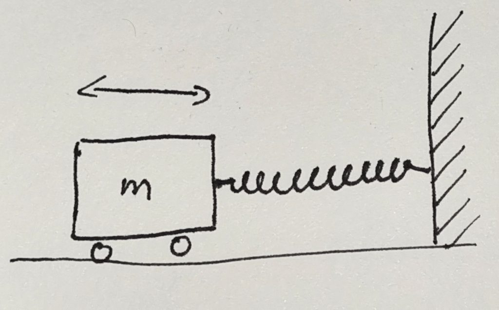
In the image, one end of the spring is attached to a wall and extends horizontally. The mass is attached to the other end and we assume that it can move without any friction. In the image, the mass has some wheels that allow it to move easily. We assume that the wheels do not create any resistance to the movement. I will come back to this assumption later.
When the system is in equilibrium, the mass will be at rest at some position along the horizontal axis. At this position, the spring does not exert any force on the mass and the mass will have no reason to move await from this equilibrium position. This is not very interesting, so let’s pull the mass away from its resting place. In what follows, I will measure the displacement, \(x\), of the mass from this equilibrium position. If we pull the mass to the right \(x\) will be positive. The spring will exert a force on the mass that will try to pull it back. The force will act towards the left, so we will assign it a negative value. A spring is designed so that the force is proportional to the displacement \(x\). The proportionality factor is called the spring constant \(k\). So we end up with a formula for the force, \[
F = -kx.
\] You can see that this formula also works if the mass is displaced to the left. In this case, \(x\) is negative and the force will be positive, pushing the mass to the right. Using the force, we can find out how the mass will move with time. The other equation that we will need for this is Newton’s law of motion, \(F = ma\) or \[
F = m \frac{d^2x}{dt^2}.
\] From these two equations we can eliminate the force and end up with \[
\frac{d^2x}{dt^2} = -\frac{k}{m}x.
\] This is a differential equation for the position \(x\). You can solve this by finding a function \(x(t)\) that, when differentiated twice, will give the same function but with a negative factor in front of it. From high school, you might remember that the \(\sin\) and \(\cos\) functions show this behavior, so let’s try it with \[
x(t) = x_0 \sin\left(\omega (t – t_0) \right).
\] Here \(x_0\), \(t_0\), and \(\omega\) are some constants that we don’t yet know. The idea is to try to keep the solution as general as possible and then see how we need to set these values to make it fit. So let’s try it out by inserting the function on both sides of our differential equation. \[
-\omega^2 x_0 \sin\left(\omega (t – t_0) \right) = -\frac{k}{m} x_0 \sin\left(\omega (t – t_0) \right).
\] Most terms in this equation cancel out and we are left with \[
\omega^2 = \frac{k}{m}.
\] This tells us that the equation of motion is satisfied whenever we choose \(\omega\) to satisfy this relation. Interestingly, the parameters \(x_0\) and \(t_0\) were canceled out which implies that we are free to choose any value for it. We could have also chosen \(\cos\) instead of \(\sin\) and ended up with the same result.
We now have a solution that depends on three parameters, \(x_0\), \(t_0\), and \(\omega\). We can do a dimensional analysis and see that \(x_0\) has units of length, \(t_0\) has units of time, and \(\omega\) is a frequency. Let’s take look at how these parameters change the behavior of the solution.
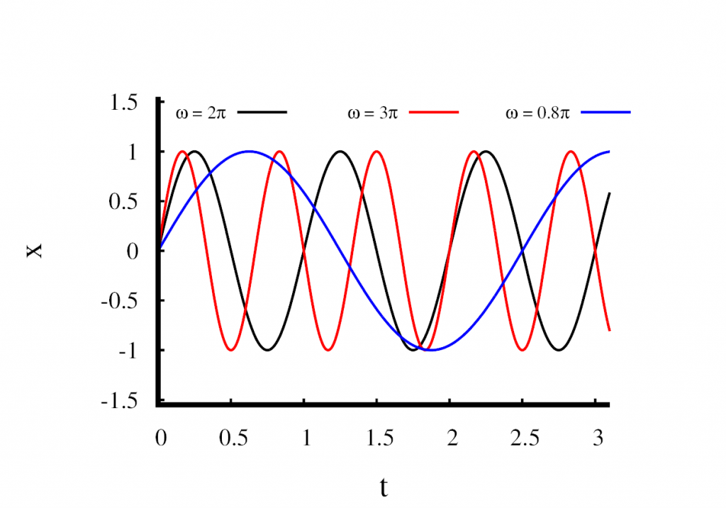
In the first figure, I have plotted three solutions in which I held \(x_0\) constant at 1m and \(t_0\) at zero. Only the parameter \(\omega\) is changed. You can see that \(\omega\) changes the speed at which the oscillations occur. A large value means that the oscillations are fast, and a small value means that the oscillations are slow. Looking at the \(\sin\) function, you can see that a full cycle finishes when the product \(\omega t\) reaches a value of \(2\pi\). This means that \(\omega\) is related to the frequency of the oscillation by \[
f = \frac{\omega}{2\pi}.
\] We call \(\omega\) the angular frequency.
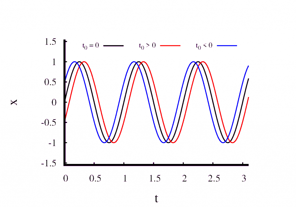
Next, have a look at what happens when we change \(t_0\) but keep all the other parameters fixed. This is shown in the second figure. You can see that \(t_0\) simply shifts the solution in time and does not modify it in any other way. We can choose \(t_0\) freely. All that this means is that we are at liberty to choose the point at which we start measuring time.
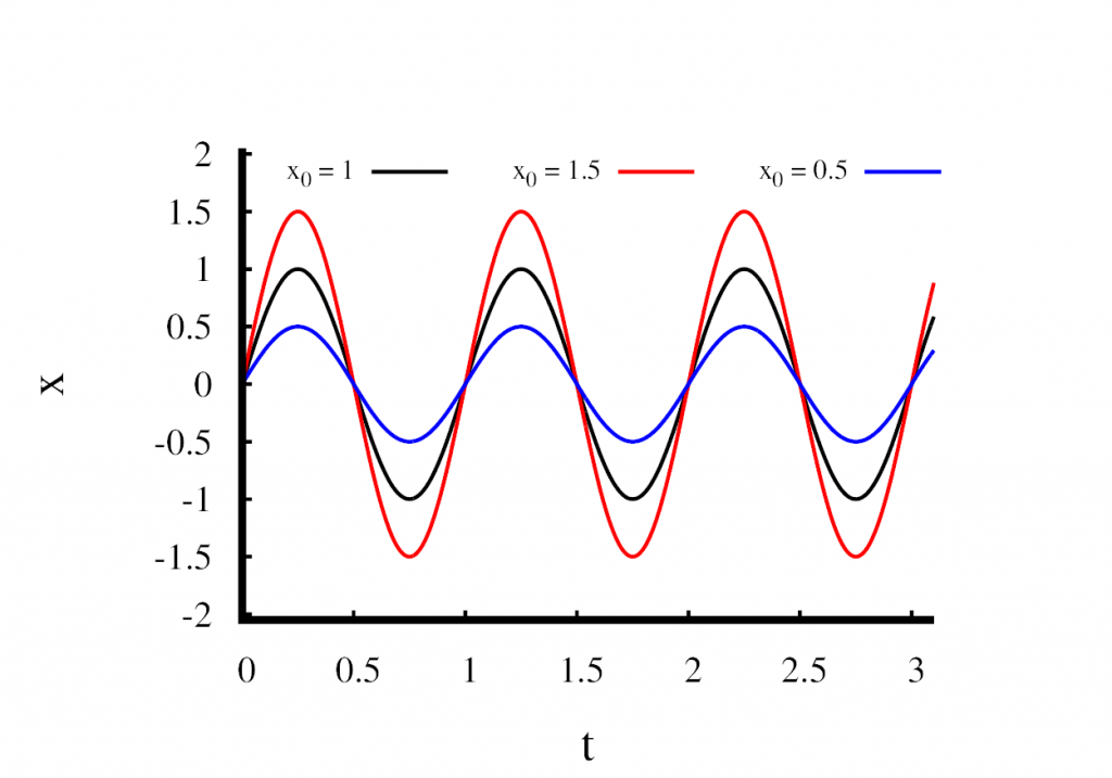
The third figure shows what happens when we modify \(x_0\) and keep all the other parameters fixed. You can clearly see that \(x_0\) changes the amplitude of the oscillation. Remember, that only the frequency \(\omega\) was fixed by the mass and the spring constant. We are free to choose \(x_0\) which means that the frequency is not influenced by our choice of \(x_0\). This leads to a very important conclusion about the harmonic oscillator.
The frequency of the oscillation is independent of its amplitude.
An energy perspective
In physics, it is often useful to look at the energy. In the spring mass system, we have two types of energy, the kinetic energy of the oscillating mass and the potential energy stored in the extended spring. We all remember the kinetic energy, \[
E_{\mathrm{kin}} = \frac{1}{2}m v^2.
\] To calculate the velocity, we have to take the derivative of the solution \(x(t)\), \[
v(t) = \omega x_0 \cos\left(\omega (t – t_0) \right).
\] The potential energy in the spring can be calculated by the work done as the spring is extended from the equilibrium length. You might remember the work to be force times distance. But in our system, the force changes with the distance. This means that the simple product has to be replaced with an integral, \[
E_{\mathrm{pot}} = \int_0^xkx\;dx = \frac{1}{2}kx^2.
\] We can take a look at the total energy over time. We know it should be constant, so let’s give it a try, \[
E_{\mathrm{tot}} = \frac{1}{2}m \omega^2 x_0^2\cos^2\left(\omega (t – t_0) \right) + \frac{1}{2}kx_0^2\sin^2\left(\omega (t – t_0) \right).
\] This can be simplified. First we can substitute \(\omega^2\) with \(k/m\). The terms in front of the trigonometric functions turn out to be the same and can be factorised, \[
E_{\mathrm{tot}} = \frac{1}{2}k x_0^2\left[\cos^2\left(\omega (t – t_0) \right) + \sin^2\left(\omega (t – t_0) \right)\right].
\] Next, Pythagoras tells us that \(\sin^2 + \cos^2 = 1\), so the bracket is just unity and we get \[
E_{\mathrm{tot}} = \frac{1}{2}k x_0^2.
\] This result confirms what we expected, the total energy is conserved and is equal to the maximum potential energy when the mass is at rest.
Another important thing to take away from this discussion is the relation between the potential energy \(E_{\mathrm{pot}} = \frac{1}{2}kx^2\) and the linear force \(F = -kx\). This relation more or less holds for any harmonic oscillator, not just the mass-and-spring system. Whenever we see a potential energy that is a parabolic function of the position, we can derive a linear force from it and we end up with a harmonic oscillator. This is why a potential of this form is also called a harmonic potential.
The oscillator in higher dimensions
The harmonic oscillator can easily be generalised to higher dimensions. Now, the displacement \(x\) is replaced by a vector \(\mathbf{r}\). The vector can be two-dimensional or three-dimensional. Then the force is also a vector and the force equation reads \[
\mathbf{F} = -k\mathbf{r}.
\] The equation states that the force always points from the position of the mass towards the origin. Just as with the one-dimensional case, the strength of the force is proportional to the distance from the origin. The force equation is relatively straightforward to grasp, but I find it slightly more instructive to look at the energy equation, \[
E_{\mathrm{pot}} = \frac{1}{2}k |\mathbf{r}|^2.
\] Let’s assume we are in three dimensions and the position vector is represented by its components \(\mathbf{r} = (x, y, z)\). We can use Pythagoras to calculate the magnitude of \(\mathbf{r}\) and end up with \[
E_{\mathrm{pot}} = \frac{1}{2}k \left(x^2 + y^2 + z^2\right).
\] Let’s write this a bit differently by expanding the bracket, \[
E_{\mathrm{pot}} = \frac{1}{2}k x^2 + \frac{1}{2}k y^2 + \frac{1}{2}k z^2.
\] You can see that this formula represents three independent harmonic oscillators. This is an important result. Imagine that the $y$ and $z$ coordinates were fixed to some value. Then the potential energy is that of a harmonic oscillator in x plus some constant offset. But it is always possible to add a constant to the potential energy because the physics only depends on potential differences. Equivalently, keeping $x$ and $z$ constant results in a harmonic oscillator in $y$.