Frege’s Numbers

Posted 19th November 2021 by Holger Schmitz

In a previous post, I started talking about natural numbers and how the Peano axioms define the relation between natural numbers. These axioms allow you to work with numbers and are good enough for most everyday uses. From a philosophical point of view, the Peano axioms have one big drawback. They only tell us how natural numbers behave but they don’t say anything about what natural numbers actually are. In the late 19th Century mathematicians started using set theory as the basis to define the axioms of arithmetic and other branches of mathematics. Two mathematicians, first Frege and later Bertrand Russell came up with a definition of natural numbers that gives us some insight into the nature of these elusive objects. In order to understand their definitions, I will first have to make the little excursion into set theory.

You may have encountered the basics of set theory already in primary school. Naïvely speaking sets are collections of things. Often the object in a set share some common property but this is not strictly necessary. You may have drawn Venn diagrams to depict sets, their unions and intersections. Something that is not taught in primary school is that you can define relations between sets that, in turn, define the so-called cardinality of a set.

Functions and Bijections

One of the central concepts is the mapping between two sets. For the following let’s assume we have two sets, \(\mathcal{A}\) and \(\mathcal{B}\). A function simply defines a rule that assigns an element of set \(\mathcal{B}\) to each element of set \(\mathcal{A}\). We call \(\mathcal{A}\) the domain of the function and \(\mathcal{B}\) the range of the function. If the function is named \(f\), then we write \[
f: \mathcal{A} \to \mathcal{B}
\] to indicate what the domain and the range of the function are.

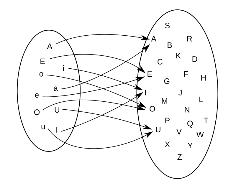
A function that maps vowels to uppercase letters

Example: For example, if \(\mathcal{A}\) is the set of uppercase and lowercase vowels, \[
\mathcal{A} = { A, E, I, O, U, a, e, i, o, u },
\] and \(\mathcal{B}\) is the set of all uppercase letters in the alphabet, \[
\mathcal{B} = { A, B, C, D, \ldots, Z}.
\]
Now we can define a function that assigns the uppercase letter in \(\mathcal{B}\) to each vowel in \(\mathcal{A}\). So the mapping looks like shown in the figure.

You will notice two properties about this function. Firstly, not all elements from \(\mathcal{B}\) appear as a mapping of an element from \(\mathcal{A}\). We say that the uppercase consonants in \(\mathcal{B}\) are not in the image of \(\mathcal{A}\).

The second thing to note is that some elements in \(\mathcal{B}\) appear twice. For example, both the lowercase e and the uppercase E in \(\mathcal{A}\) map to the same uppercase E in \(\mathcal{B}\).

Definition of a Bijection

The example shows a function that is not a bijection. In order to be a bijection, a function must ensure that each element in the range is mapped to by exactly one element from the range. In other words for a function \[
f: \mathcal{A} \to \mathcal{B}
\]

• every element in \(\mathcal{B}\) appears as a function value. No element is left out.
• no element in \(\mathcal{B}\) appears as a function value more than once.

A bijection implies a one-to-one relationship between the elements in set \(\mathcal{A}\) and set \(\mathcal{B}\).

Equinumerosity and Cardinality

Intuitively, it is clear that you can only have a bijection between two sets if they have the same number of elements. After all, each element in \(\mathcal{A}\) is mapped onto exactly one element in \(\mathcal{B}\). This can be used to define a relation between any two sets.

Two sets are called equinumerous if there exists a bijection between the two sets. Equinumerous literally means “having the same number”. But we have to be careful here because we don’t yet know what the term “number” is supposed to mean. That is the reason why we define the term by using bijections and not referring to any “amount” or “number of elements”. Instead of saying that two sets are equinumerous, we can also say that they have the same cardinality.

Now comes the clever bit that Frege proposed. Let’s create a class of sets that all share the same cardinality. We can do that because equinumerosity is an equivalence relation but I won’t go into detail about what that means. We will call this cardinality class \(N\), so \[
N(\mathcal{A})
\] is the class of all the sets that are equinumerous to \(\mathcal{A}\).

Intuitively we now have a class with all the sets that contain exactly one element, another class with all the sets that contain exactly two elements, and so forth. But we don’t know anything about numbers yet, so we also don’t really know what one and two are supposed to mean.

Constructing Natural Numbers

Now we have all the tools to construct the natural numbers \(\mathbb{N}\). Of course, we want our numbers to obey the Peano axioms, so we need two things. We need a zero element and we need a successor function \(S(n)\) that produces the next number from any given number.

The Zero Element

The zero-element is easily defined. We can construct the empty set, \[
\emptyset = \{\}.
\] This is the set with no elements in it. Now the zero-element is simply the cardinality class of the empty set, \[
0 = N(\emptyset).
\] This means that zero is a class of sets that all share the same cardinality as the empty set. You can show that this class consists of only one element, the empty set, by I won’t go into that here.

The Successor Function

Given that we have defined the zero element, \(0\), we can now define a set that contains zero as a single element, \[
\{0\}.
\] Intuitively, this set has one element and we can thus define the natural number \(1\) as the cardinality class of this set, \[
1 = N(\{0\}).
\] In general, given any natural number \(n\) we can define the successor \(S(n)\) by creating the cardinality class of the set that contains \(n\) together with all its predecessors, \[
n+1 = S(n) = N(\{0, 1, \ldots, n\}).
\] You might think that this definition is somewhat circular. We are defining the successor function by using the concept of the predecessors. But this is not as problematic as it might seem at first sight. We know that the predecessor of \(1\) is \(0\) and each time we construct the next natural number, we can keep track of all the predecessors that we have constructed so far.

Conclusion

The zero and the successor function defined above are enough to define all the natural numbers \(\mathbb{N}\). I will not go into the proof that all the Peano axioms are satisfied by this construction. It is relatively straightforward and not very instructive in my opinion. If you want, you can try doing the proof as an exercise.

I personally find the Frege definition of natural numbers the most satisfying. It tells us that a number is not just some random symbol that doesn’t relate to the real world. A natural number is the class of all sets that share the same property. Each set in the class has the same cardinality and we can identify the cardinality with that number. It means that any set of objects in the real world can be thought of as an instance of a number. The number itself is the collection of sets and the concrete set is contained within it as an element. For example, if you see five apples on a table, you can think of them as a manifestation of the number \(5\).

This set of pins is an instance of the number 4 (four).

Another consequence of the definition of cardinality is that it gives us the ability to speak about infinities. A set might have an infinite number of elements. We already encountered \(\mathbb{N}\), the set of all natural numbers. Using the cardinality, we can compare infinite sets and create a hierarchy of infinities. I might talk about this more in a later post.

It would not be fair, however, if I didn’t mention some serious problems with the definition that I Frege came up with. The main problem arises because we are creating classes of sets without explicitly saying which elements we are allowing to be in those sets. This allows sets to contain arbitrary elements, including other sets. A set can even include itself as an element. This leads to the famous paradox by Russel which can be summarised as follows. Construct a set \(\mathcal{R}\) of all the sets that do not include themselves as an element. Then ask the question, does \(\mathcal{R}\) include itself? There are mathematical frameworks that attempt to save the essence of Frege’s definition of the natural numbers without running into these problems. In my personal opinion, they always lose some of the beauty and simplicity. But this is a necessary concession to make if you want to end up with a mathematical framework that doesn’t contain internal contradictions.

Read More

Computational Physics Basics: Accuracy and Precision

Posted 24th August 2021 by Holger Schmitz

Problems in physics almost always require us to solve mathematical equations with real-valued solutions, and more often than not we want to find functional dependencies of some quantity of a real-valued domain. Numerical solutions to these problems will only ever be approximations to the exact solutions. When a numerical outcome of the calculation is obtained it is important to be able to quantify to what extent it represents the answer that was sought. Two measures of quality are often used to describe numerical solutions: accuracy and precision. Accuracy tells us how will a result agrees with the true value and precision tells us how reproducible the result is. In the standard use of these terms, accuracy and precision are independent of each other.

Accuracy

Accuracy refers to the degree to which the outcome of a calculation or measurement agrees with the true value. The technical definition of accuracy can be a little confusing because it is somewhat different from the everyday use of the word. Consider a measurement that can be carried out many times. A high accuracy implies that, on average, the measured value will be close to the true value. It does not mean that each individual measurement is near the true value. There can be a lot of spread in the measurements. But if we only perform the measurement often enough, we can obtain a reliable outcome.

Precision

Precision refers to the degree to which multiple measurements agree with each other. The term precision in this sense is orthogonal to the notion of accuracy. When carrying out a measurement many times high precision implies that the outcomes will have a small spread. The measurements will be reliable in the sense that they are similar. But they don’t necessarily have to reflect the true value of whatever is being measured.

Accuracy vs Precision

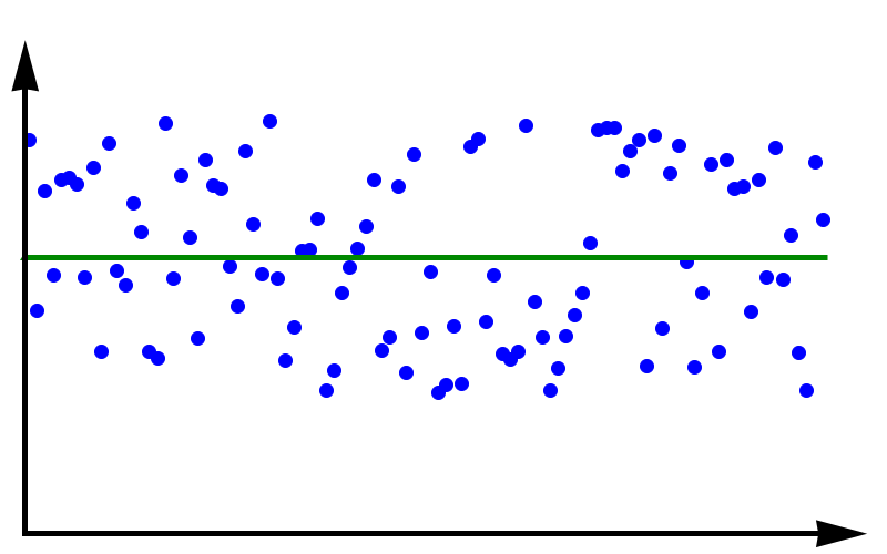
Data with high accuracy but low precision. The green line represents the true value.

To fully grasp the concept of accuracy vs precision it is helpful to look at these two plots. The crosses represent measurements whereas the line represents the true value. In the plot above, the measurements are spread out but they all lie around the true value. These measurements can be said to have low precision but high accuracy. In the plot below, all measurements agree with each other, but they do not represent the true value. In this case, we have high precision but low accuracy.

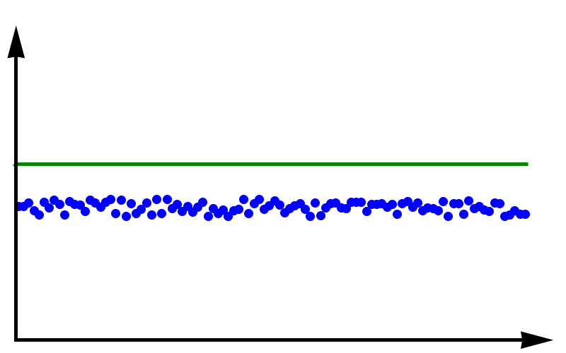
Data with high precision but low accuracy. The green line represents the true value.

A moral can be gained from this: just because you always get the same answer doesn’t mean the answer is correct.

When thinking about numerical methods you might object that calculations are deterministic. Therefore the outcome of repeating a calculation will always be the same. But there is a large class of algorithms that are not quite so deterministic. They might depend on an initial guess or even explicitly on some sequence of pseudo-random numbers. In these cases, repeating the calculation with a different guess or random sequence will lead to a different result.

Read More

What are Numbers? Or, Learning to Count!

Posted 17th April 2021 by Holger Schmitz

We all use numbers every day and some of us feel more comfortable dealing with them than others. But have you ever asked yourself what numbers really are? For example, what is the number 4? Of course, you can describe the symbol “4”. But that is not really the number, is it? You can use Roman numerals IV, Urdu ۴, or Chinese and Japanese Kanji 四. Each one of these symbols represents the same number. And yet, somehow we would all probably agree that there is only one number 4.

The question about the nature of numbers is twofold. You can understand this question purely mathematical one and ask for a clear definition of a number and the set of numbers in a mathematical sense. This will be the topic of this article. You can also ask yourself what numbers are in a philosophical sense. Do numbers exist? If yes, in what way do they exist, and what are they? This may be the topic of a future article.

Now that we have settled what type of question we want to answer, we should start with the simplest type of numbers. These are the natural numbers 0, 1, 2, 3, 4, …
I decided to include the number zero even though it might seem a little abstract at first. After all, what does it mean to have zero of something? But that objection strays into the philosophical realm again and, as I said above, I want to focus on the mathematical aspect here.

When doing the research for this article, I was slightly surprised at the plethora of different definitions for the natural numbers. But given how fundamental this question is, it should be no wonder that many mathematicians have thought about the problem of defining numbers and have come up with different answers.

The Peano Axioms

Let’s start with an axiomatic definition of numbers called the Peano axioms. This is one of the earliest strict definitions of the natural numbers in the modern sense. It doesn’t really state what the natural numbers are but focuses on how they behave. We start with the set of natural numbers, which we call $\mathbb{N}$, and a successor function $S$.

Peano Axiom 1:

$0$ is a natural number or, more formally, $0 \in \mathbb{N}$

This axiom just tells us that there is a natural number zero. We could have chosen 1 as the starting point but this is arbitrary.

Peano Axiom 2:

Every natural number $x$ has a successor $y$.
In other words, given that $x \in \mathbb{N}$ then it follows that $y = S(x) \in \mathbb{N}$.

Intuitively, the successor function will always produce the next natural number.
Mathematicians call this property of the natural number being closed under the successor operation $S$. All this means is that the successor operation will never produce a result that is outside of the natural numbers.

Peano Axiom 3:

If we have two natural numbers $x$ and $y$, and we know that the successors of $x$ and $y$ are equal, then this is the same as saying that $x$ and $y$ are equal.
Again, written more formally we say, given $x \in \mathbb{N}$ and $y \in \mathbb{N}$ and $S(x) = S(y)$ then it follows that $x=y$.

This means that any natural number cannot be the successor of two different number. In other words, if you have two different numbers then they can’t have the same successor.

Peano Axiom 4:

$0$ is not the successor of any other natural number.
In mathematical notation, if $x \in \mathbb{N}$ then $S(x) \ne 0$

At first sight, we might think that these axioms are complete. We can start from zero and use the successor function $S$ to iterate through the natural numbers. This is intuitively shown in the image below.

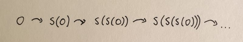
Repeatedly applying the successor function, starting from 0.

Here
1 = S(0)
2 = S(S(0)) = S(1)
3 = S(S(S(0))) = S(2)
and so on.

But we haven’t guaranteed that this iteration will eventually be able to reach all natural numbers. Imagine that, in addition to the above, there is some special number $z$ that creates a closed loop when applying the successor function. And this loop is separate from the sequence that we get when starting from zero.

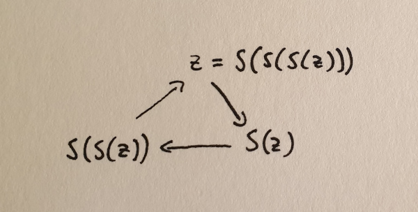
A closed loop of successors that isn’t connected to the zero element.

So we need another axiom that guarantees that all natural numbers are reachable from zero by repeatedly applying the successor function. This axiom is usually stated in the following way.

Peano Axiom 5: Axiom of Induction

Given any set $U \subseteq \mathbb{N}$ with $0 \in U$.
If $U$ is such that for every $n \in U$ the successor is also in $U$, i.e. $S(n) \in U$,
then $U = \mathbb{N}$

The idea behind this axiom is that $U$ can be chosen as the minimal set that contains no additional loops or numbers that are not reachable from zero. The fact that any set $U$ that contains zero and is closed under the successor function is identical to the natural numbers guarantees that all natural numbers are eventually reachable from zero. The axiom of induction is maybe more familiar in its alternative form.

Peano Axiom 5: Axiom of Induction, alternative form

Consider a mathematical statement that is true for zero.
If it can be proven that,
given the statement is true for a number $n$, then it is also true for $S(n)$,
then it follows that the statement is true for all natural numbers.

Here you can see that this axiom forms the basis of the familiar proof by induction.

Some Remarks

The Peano Axioms are helpful in defining the set of natural numbers $\mathbb{N}$ and arithmetic operations on them. But personally, I feel unsatisfied by this definition. The Peano Axioms tell us how natural numbers behave but they don’t really give any additional insight as to what numbers really are.

Take for example the number 2. We now know that 2 can be expressed as the successor of the successor of 0, i.e. $2 = S(S(0))$. We also know that this second successor must be a member of the set of natural numbers, but not much more. The problem here is that we never defined what the successor function should be.

Nonetheless, the Peano axioms can serve as a basis for more in-depth definitions of the natural numbers. These definitions can be considered models of the Peano Axioms in the sense that they define a zero element and some concrete successor function. The set of natural numbers can then be constructed from these and the Peano Axioms follow as consequences from these definitions.

In a future post, I will look at some set-theoretic definitions of the natural numbers. If you liked this post, please leave a comment and check back soon for more content.

Read More

Computational Physics Basics: Integers in C++, Python, and JavaScript

Posted 5th August 2020 by Holger Schmitz

In a previous post, I wrote about the way that the computer stores and processes integers. This description referred to the basic architecture of the processor. In this post, I want to talk about how different programming languages present integers to the developer. Programming languages add a layer of abstraction and in different languages that abstraction may be less or more pronounced. The languages I will be considering here are C++, Python, and JavaScript.

Integers in C++

C++ is a language that is very close to the machine architecture compared to other, more modern languages. The data that C++ operates on is stored in the machine’s memory and C++ has direct access to this memory. This means that the C++ integer types are exact representations of the integer types determined by the processor architecture.

The following integer datatypes exist in C++

This table does not give the exact size of the datatypes because the C++ standard does not specify the sizes but only lower limits. It is also required that the larger types must not use fewer bits than the smaller types. The exact number of bits used is up to the compiler and may also be changed by compiler options. To find out more about the regular integer types you can look at this reference page.

The reason for not specifying exact sizes for datatypes is the fact that C++ code will be compiled down to machine code. If you compile your code on a 16 bit processor the plain int type will naturally be limited to 16 bits. On a 64 bit processor on the other hand, it would not make sense to have this limitation.

Each of these datatypes is signed by default. It is possible to add the signed qualifier before the type name to make it clear that a signed type is being used. The unsigned qualifier creates an unsigned variant of any of the types. Here are some examples of variable declarations.

char c; // typically 8 bit
unsigned int i = 42; // an unsigned integer initialised to 42
signed long l; // the same as "long l" or "long int l"

As stated above, the C++ standard does not specify the exact size of the integer types. This can cause bugs when developing code that should be run on different architectures or compiled with different compilers. To overcome these problems, the C++ standard library defines a number of integer types that have a guaranteed size. The table below gives an overview of these types.

More details on these and similar types can be found here.

The code below prints a 64 bit int64_t using the binary notation. As the name suggests, the bitset class interprets the memory of the data passed to it as a bitset. The bitset can be written into an output stream and will show up as binary data.

#include  <bitset>

void printBinaryLong(int64_t num) {
    std::cout << std::bitset<64>(num) << std::endl;
}

Integers in Python

Unlike C++, Python hides the underlying architecture of the machine. In order to discuss integers in Python, we first have to make clear which version of Python we are talking about. Python 2 and Python 3 handle integers in a different way. The Python interpreter itself is written in C which can be regarded in many ways as a subset of C++. In Python 2, the integer type was a direct reflection of the long int type in C. This meant that integers could be either 32 or 64 bit, depending on which machine a program was running on.

This machine dependence was considered bad design and was replaced be a more machine independent datatype in Python 3. Python 3 integers are quite complex data structures that allow storage of arbitrary size numbers but also contain optimizations for smaller numbers.

It is not strictly necessary to understand how Python 3 integers are stored internally to work with Python but in some cases it can be useful to have knowledge about the underlying complexities that are involved. For a small range of integers, ranging from -5 to 256, integer objects are pre-allocated. This means that, an assignment such as

n = 25

will not create the number 25 in memory. Instead, the variable n is made to reference a pre-allocated piece of memory that already contained the number 25. Consider now a statement that might appear at some other place in the program.

a = 12
b = a + 13

The value of b is clearly 25 but this number is not stored separately. After these lines b will reference the exact same memory address that n was referencing earlier. For numbers outside this range, Python 3 will allocate memory for each integer variable separately.

Larger integers are stored in arbitrary length arrays of the C int type. This type can be either 16 or 32 bits long but Python only uses either 15 or 30 bits of each of these "digits". In the following, 32 bit ints are assumed but everything can be easily translated to 16 bit.

Numbers between −(2³⁰ − 1) and 2³⁰ − 1 are stored in a single int. Negative numbers are not stored as two’s complement. Instead the sign of the number is stored separately. All mathematical operations on numbers in this range can be carried out in the same way as on regular machine integers. For larger numbers, multiple 30 bit digits are needed. Mathamatical operations on these large integers operate digit by digit. In this case, the unused bits in each digit come in handy as carry values.

Integers in JavaScript

Compared to most other high level languages JavaScript stands out in how it deals with integers. At a low level, JavaScript does not store integers at all. Instead, it stores all numbers in floating point format. I will discuss the details of the floating point format in a future post. When using a number in an integer context, JavaScript allows exact integer representation of a number up to 53 bit integer. Any integer larger than 53 bits will suffer from rounding errors because of its internal representation.

const a = 25;
const b = a / 2;

In this example, a will have a value of 25. Unlike C++, JavaScript does not perform integer divisions. This means the value stored in b will be 12.5.

JavaScript allows bitwise operations only on 32 bit integers. When a bitwise operation is performed on a number JavaScript first converts the floating point number to a 32 bit signed integer using two’s complement. The result of the operation is subsequently converted back to a floating point format before being stored.

Read More