Computational Physics Basics: Polynomial Interpolation
Posted 19th April 2023 by Holger Schmitz
The piecewise constant interpolation and the linear interpolation seen in the previous post can be understood as special cases of a more general interpolation method. Piecewise constant interpolation constructs a polynomial of order 0 that passes through a single point. Linear interpolation constructs a polynomial of order 1 that passes through 2 points. We can generalise this idea to construct a polynomial of order \(n-1\) that passes through \(n\) points, where \(n\) is 1 or greater. The idea is that a higher-order polynomial will be better at approximating the exact function. We will see later that this idea is only justified in certain cases and that higher-order interpolations can actually increase the error when not applied with care.
Existence
The first question that arises is the following. Given a set of \(n\) points, is there always a polynomial of order \(n-1\) that passes through these points, or are there multiple polynomials with that quality? The first question can be answered simply by constructing a polynomial. The simplest way to do this is to construct the Lagrange Polynomial. Assume we are given a set of points, \[
(x_1, y_1), (x_2, y_2) \ldots (x_n, y_n),
\] where all the \(x\)’s are different, i.e. \(x_i \ne x_j\) if \(i \ne j\). Then we observe that the fraction \[
\frac{x – x_j}{x_i – x_j}
\] is zero when \(x = x_j\) and one when \(x = x_i\). Next, let’s choose an index \(i\) and multiply these fractions together for all \(j\) that are different to \(i\), \[
a_i(x) = \frac{x – x_1}{x_i – x_1}\times \ldots\times\frac{x – x_{i-1}}{x_i – x_{i-1}}
\frac{x – x_{i+1}}{x_i – x_{i+1}}\times \ldots\times\frac{x – x_n}{x_i – x_n}.
\] This product can be written a bit more concisely as \[
a_i(x) = \prod_{\stackrel{j=1}{j\ne i}}^n \frac{x – x_j}{x_i – x_j}.
\] You can see that the \(a_i\) are polynomials of order \(n-1\). Now, if \(x = x_i\) all the factors in the product are 1 which means that \(a_i(x_i) = 1\). On the other hand, if \(x\) is any of the other \(x_j\) then one of the factors will be zero and \(a_i(x_j) = 0\) for any \(j \ne i\). Thus, if we take the product \(a_i(x) y_i\) we have a polynomial that passes through the point \((x_i, y_i)\) but is zero at all the other \(x_j\). The final step is to add up all these separate polynomials to construct the Lagrange Polynomial, \[
p(x) = a_1(x)y_1 + \ldots a_n(x)y_n = \sum_{i=1}^n a_i(x)y_i.
\] By construction, this polynomial of order \(n-1\) passes through all the points \((x_i, y_i)\).
Uniqueness
The next question is if there are other polynomials that pass through all the points, or is the Lagrange Polynomial the only one? The answer is that there is exactly one polynomial of order \(n\) that passes through \(n\) given points. This follows directly from the fundamental theorem of algebra. Imagine we have two order \(n-1\) polynomials, \(p_1\) and \(p_2\), that both pass through our \(n\) points. Then the difference, \[
d(x) = p_1(x) – p_2(x),
\] will also be an order \(n-1\) degree polynomial. But \(d\) also has \(n\) roots because \(d(x_i) = 0\) for all \(i\). But the fundamental theorem of algebra asserts that a polynomial of degree \(n\) can have at most \(n\) real roots unless it is identically zero. In our case \(d\) is of order \(n-1\) and should only have \(n-1\) roots. The fact that it has \(n\) roots means that \(d \equiv 0\). This in turn means that \(p_1 = p_2\) must be the same polynomial.
Approximation Error and Runge’s Phenomenon
One would expect that the higher order interpolations will reduce the error of the approximation and that it would always be best to use the highest possible order. One can find the upper bounds of the error using a similar approach that I used in the previous post on linear interpolation. I will not show the proof here, because it is a bit more tedious and doesn’t give any deeper insights. Given a function \(f(x)\) over an interval \(a\le x \le b\) and sampled at \(n+1\) equidistant points \(x_i = a + hi\), with \(i=0, \ldots , n+1\) and \(h = (b-a)/n\), then the order \(n\) Lagrange polynomial that passes through the points will have an error given by the following formula. \[
\left|R_n(x)\right| \leq \frac{h^{n+1}}{4(n+1)} \left|f^{(n+1)}(x)\right|_{\mathrm{max}}
\] Here \(f^{(n+1)}(x)\) means the \((n+1)\)th derivative of the the function \(f\) and the \(\left|.\right|_{\mathrm{max}}\) means the maximum value over the interval between \(a\) and \(b\). As expected, the error is proportional to \(h^{n+1}\). At first sight, this implies that increasing the number of points, and thus reducing \(h\) while at the same time increasing \(n\) will reduce the error. The problem arises, however, for some functions \(f\) whose \(n\)-th derivatives grow with \(n\). The example put forward by Runge is the function \[
f(x) = \frac{1}{1+25x^2}.
\]
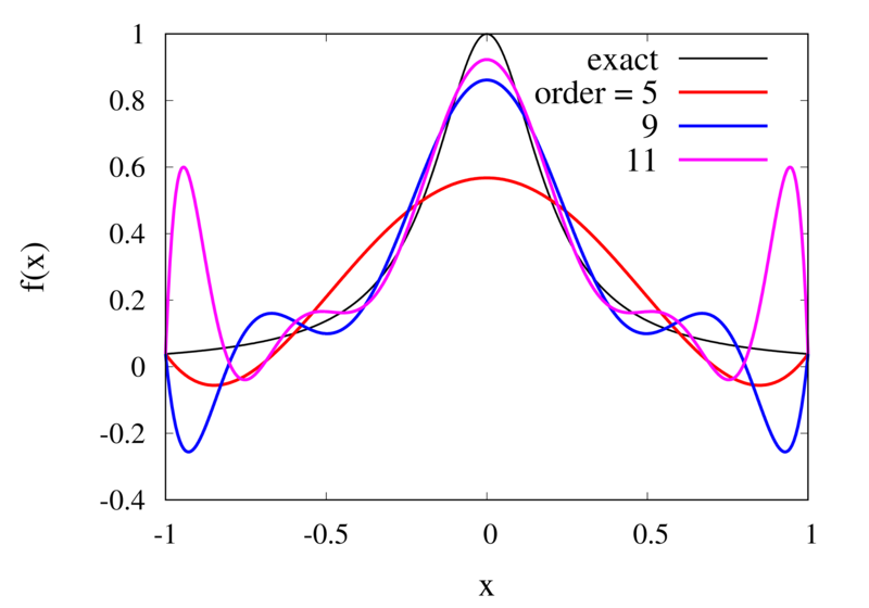
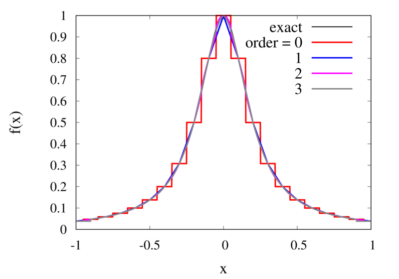
Interpolation of Runge’s function using higher-order polynomials.
The figure above shows the Lagrange polynomials approximating Runge’s function over the interval from -1 to 1 for some orders. You can immediately see that the approximations tend to improve in the central part as the order increases. But near the outermost points, the Lagrange polynomials oscillate more and more wildly as the number of points is increased. The conclusion is that one has to be careful when increasing the interpolation order because spurious oscillations may actually degrade the approximation.
Piecewise Polynomial Interpolation
Does this mean we are stuck and that moving to higher orders is generally bad? No, we can make use of higher-order interpolations but we have to be careful. Note, that the polynomial interpolation does get better in the central region when we decrease the spacing between the points. When we used piecewise linear of constant interpolation, we chose the points that were used for the interpolation based on where we wanted to interpolate the function. In the same way, we can choose the points through which we construct the polynomial so that they are always symmetric around \(x\). Some plots of this piecewise polynomial interpolation are shown in the plot below.
Piecewise Lagrange interpolation with 20 points for orders 0, 1, 2, and 3.
Let’s analyse the error of these approximations. Using an array with \(N\) points on Runge’s function equally spaced between -2 and 2. \(N\) was varied between 10 and 10,000. For each \(N\), the centred polynomial interpolation of orders 0, 1, 2, and 3 was created. Finally, the maximum error of the interpolation and the exact function over the interval -1 and 1 are determined.
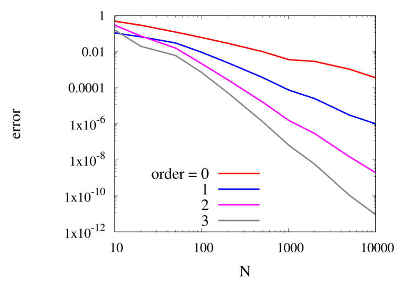
Scaling of the maximum error of the Lagrange interpolation with the number of points for increasing order.
The plot above shows the double-logarithmic dependence of the error against the number of points for each order interpolation. The slope of each curve corresponds to the order of the interpolation. For the piecewise constant interpolation, an increase in the number of points by 3 orders of magnitude also corresponds to a reduction of the error by three orders of magnitude. This indicates that the error is first order in this case. For the highest order interpolation and 10,000 points, the error reaches the rounding error of double precision.
Discontinuities and Differentiability
As seen in the previous section, for many cases the piecewise polynomial interpolation can provide a good approximation to the underlying function. However, in some cases, we need to use the first or second derivative of our interpolation. In these cases, the Lagrange formula is not ideal. To see this, the following image shows the interpolation error, again for Runge’s function, using order 2 and 3 polynomials and 20 points.
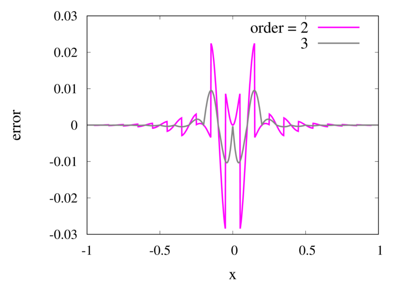
Error in the Lagrange interpolation of Runge’s function for orders 2 and 3.
One can see that the error in the order 2 approximation has discontinuities and the error in the order 3 approximation has discontinuities of the derivative. For odd-order interpolations, the points that are used for the interpolation change when \(x\) moves from an interval \([x_{i-1},x_i]\) to an interval \([x_i, x_{i+1}]\). Because both interpolations are the same at the point \(x_i\) itself, the interpolation is continuous but the derivative, in general, is not. For even-order interpolations, the stencil changes halfway between the points, which means that the function is discontinuous there. I will address this problem in a future post.
Computational Physics Basics: Piecewise and Linear Interpolation
Posted 24th February 2022 by Holger Schmitz
One of the main challenges of computational physics is the problem of representing continuous functions in time and space using the finite resources supplied by the computer. A mathematical function of one or more continuous variables naturally has an infinite number of degrees of freedom. These need to be reduced in some manner to be stored in the finite memory available. Maybe the most intuitive way of achieving this goal is by sampling the function at a discrete set of points. We can store the values of the function as a lookup table in memory. It is then straightforward to retrieve the values at the sampling points. However, in many cases, the function values at arbitrary points between the sampling points are needed. It is then necessary to interpolate the function from the given data.
Apart from the interpolation problem, the pointwise discretisation of a function raises another problem. In some cases, the domain over which the function is required is not known in advance. The computer only stores a finite set of points and these points can cover only a finite domain. Extrapolation can be used if the asymptotic behaviour of the function is known. Also, clever spacing of the sample points or transformations of the domain can aid in improving the accuracy of the interpolated and extrapolated function values.
In this post, I will be talking about the interpolation of functions in a single variable. Functions with a higher-dimensional domain will be the subject of a future post.
Functions of a single variable
A function of a single variable, \(f(x)\), can be discretised by specifying the function values at sample locations \(x_i\), where \(i=1 \ldots N\). For now, we don’t require these locations to be evenly spaced but I will assume that they are sorted. This means that \(x_i < x_{i+1}\) for all \(i\). Let’s define the function values, \(y_i\), as \[
y_i = f(x_i).
\] The intuitive idea behind this discretisation is that the function values can be thought of as a number of measurements. The \(y_i\) provide incomplete information about the function. To reconstruct the function over a continuous domain an interpolation scheme needs to be specified.
Piecewise Constant Interpolation
The simplest interpolation scheme is the piecewise constant interpolation, also known as the nearest neighbour interpolation. Given a location \(x\) the goal is to find a value of \(i\) such that \[
|x-x_i| \le |x-x_j| \quad \text{for all} \quad j\ne i.
\] In other words, \(x_i\) is the sample location that is closest to \(x\) when compared to the other sample locations. Then, define the interpolation function \(p_0\) as \[
p_0(x) = f(x_i)
\] with \(x_i\) as defined above. The value of the interpolation is simply the value of the sampled function at the sample point closest to \(x\).
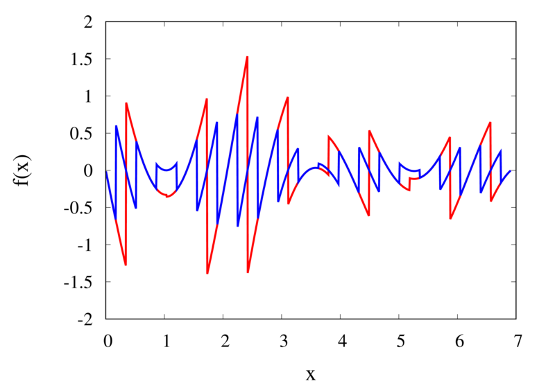
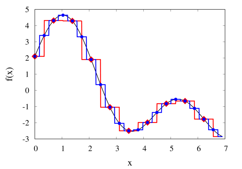
Piecewise constant interpolation of a function (left) and the error (right)
The left plot in the figure above shows some smooth function in black and a number of sample points. The case where 10 sample points are taken is shown by the diamonds and the case for 20 sample points is shown by the circles. Also shown are the nearest neighbour interpolations for these two cases. The red curve shows the interpolated function for 10 samples and the blue curve is for the case of 20 samples. The right plot in the figure shows the difference between the original function and the interpolations. Again, the red curve is for the case of 10 samples and the blue curve is for the case of 20 samples. We can see that the piecewise constant interpolation is crude and the errors are quite large.
As expected, the error is smaller when the number of samples is increased. To analyse exactly how big the error is, consider the residual for the zero-order interpolation \[
R_0(x) = f(x) – p_0(x) = f(x) – f(x_i).
\] The first step to analyse the magnitude of the residual is to perform a Taylor expansion of the residual around the point \(x_i\). We only need the zero order term. Using Taylor’s Theorem and the Cauchy form of the remainder, one can write \[
R_0(x) = \left[ f(x_i) + f'(\xi_c)(x – x_i)\right] – f(x_i).
\] The term in the brackets is the Taylor expansion of \(f(x)\), and \(\xi_c\) is some value that lies between \(x_i\) and \(x\) and depends on the value of \(x\). Let’s define the distance between two samples with \(h=x_{i+1}-x_i\). Assume for the moment that all samples are equidistant. It is not difficult to generalise the arguments for the case when the support points are not equidistant. This means, the maximum value of \(x – x_i\) is half of the distance between two samples, i.e. \[
x – x_i \le \frac{h}{2}.
\] It os also clear that \(f'(\xi_c) \le |f'(x)|_{\mathrm{max}}\), where the maximum is over the interval \(|x-x_i| \le h/2\). The final result for an estimate of the residual error is \[
|R_0(x)| \le\frac{h}{2} |f'(x)|_{\mathrm{max}}
\]
Linear Interpolation
As we saw above, the piecewise interpolation is easy to implement but the errors can be quite large. Most of the time, linear interpolation is a much better alternative. For functions of a single argument, as we are considering here, the computational expense is not much higher than the piecewise interpolation but the resulting accuracy is much better. Given a location \(x\), first find \(i\) such that \[
x_i \le x < x_{i+1}.
\] Then the linear interpolation function \(p_1\) can be defined as \[
p_1(x) = \frac{x_{i+1} – x}{x_{i+1} – x_i} f(x_i)
+ \frac{x – x_i}{x_{i+1} – x_i} f(x_{i+1}).
\] The function \(p_1\) at a point \(x\) can be viewed as a weighted average of the original function values at the neighbouring points \(x_i\) and \(x_{i+1}\). It can be easily seen that \(p(x_i) = f(x_i)\) for all \(i\), i.e. the interpolation goes through the sample points exactly.
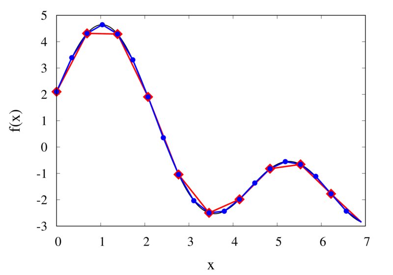
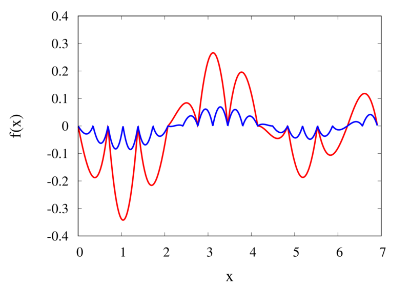
Linear interpolation of a function (left) and the error (right)
The left plot in the figure above shows the same function \(f(x)\) as the figure in the previous section but now together with the linear interpolations for 10 samples (red curve) and 20 samples (blue curve). One can immediately see that the linear interpolation resembles the original function much more closely. The right plot shows the error for the two interpolations. The error is much smaller when compared to the error for the piecewise interpolation. For the 10 sample interpolation, the maximum absolute error of the linear interpolation is about 0.45 compared to a value of over 1.5 for the nearest neighbour interpolation. What’s more, going from 10 to 20 samples improves the error substantially.
One can again try to quantify the error of the linear approximation using Taylor’s Theorem. The first step is to use the Mean Value Theorem that states that there is a point \(x_c\) between \(x_i\) and \(x_{i+1}\) that satisfies \[
f'(x_c) = \frac{ f(x_{i+1}) – f(x_i) }{ x_{i+1} – x_i }.
\] Consider now the error of the linear approximation, \[
R_1(x) = f(x) – p_1(x) = f(x) – \left[\frac{x_{i+1} – x}{x_{i+1} – x_i} f(x_i)
+ \frac{x – x_i}{x_{i+1} – x_i} f(x_{i+1})\right].
\] The derivative of the error is \[
R’_1(x) = f'(x) – \frac{ f(x_{i+1}) – f(x_i) }{ x_{i+1} – x_i }.
\] The Mean Value Theorem implies that the derivative of the error at \(x_c\) is zero and the error is at its maximum at that point. In other words, to estimate the maximum error, we only need to find an upper bound of \(|R(x_c)|\).
We now perform a Taylor expansion of the error around \(x_c\). Using again the Cauchy form of the remainder, we find \[
R(x) = R(x_c) + xR'(x_c) + \frac{1}{2}R’^\prime(\xi_c)(x-\xi_c)(x-x_c).
\] The second term on the right hand side is zero by construction, and we have \[
R(x) = R(x_c) + \frac{1}{2}R’^\prime(\xi_c)(x-\xi_c)(x-x_c).
\] Let \(h\) again denote the distance between the two points, \(h=x_{i+1} – x_i\). We assume that \(x_c – x_i < h/2\) and use the equation above to calculate \(R(x_i)\) which we know is zero. If \(x_c\) was closer to \(x_{i+1}\) we would have to calculate \(R(x_{i+1})\) but otherwise the argument would remain the same. So, \[
R(x_i) = 0 = R(x_c) + \frac{1}{2}R’^\prime(\xi_c)(x_i-\xi_c)(x_i-x_c)
\] from which we get \[
|R(x_c)| = \frac{1}{2}|R’^\prime(\xi_c)(x_i-\xi_c)(x_i-x_c)|.
\] To get an upper estimate of the remainder that does not depend on \(x_c\) or \(\xi_c\) we can use the fact that both \(x_i-\xi_c \le h/2\) and \(x_i-x_c \le h/2\). We also know that \(|R(x)| \le |R(x_c)|\) over the interval from \(x_i\) to \(x_{i+1}\) and \(|R’^\prime(\xi_c)| = |f’^\prime(\xi_c)| \le |f’^\prime(x)|_{\mathrm{max}}\). Given all this, we end up with \[
|R(x)| \le \frac{h^2}{8}|f’^\prime(x)|_{\mathrm{max}}.
\]
The error of the linear interpolation scales with \(h^2\), in contrast to \(h\) for the piecewise constant interpolation. This means that increasing the number of samples gives us much more profit in terms of accuracy. Linear interpolation is often the method of choice because of its relative simplicity combined with reasonable accuracy. In a future post, I will be looking at higher-order interpolations. These higher-order schemes will scale even better with the number of samples but this improvement comes at a cost. We will see that the price to be paid is not only a higher computational expense but also the introduction of spurious oscillations that are not present in the original data.
The Harmonic Oscillator
Posted 11th February 2022 by Holger Schmitz
I wasn’t really planning on writing this post. I was preparing a different post when I found that I needed to explain a property of the so-called “harmonic oscillator”. I first thought about adding a little excursion into the article that I was going to write. But I found that the harmonic oscillator is such an important concept in physics that it would not be fair to deny it its own post. The harmonic oscillator appears in many contexts and I don’t think there is any branch in physics that can do without it.
The Spring-and-Mass System
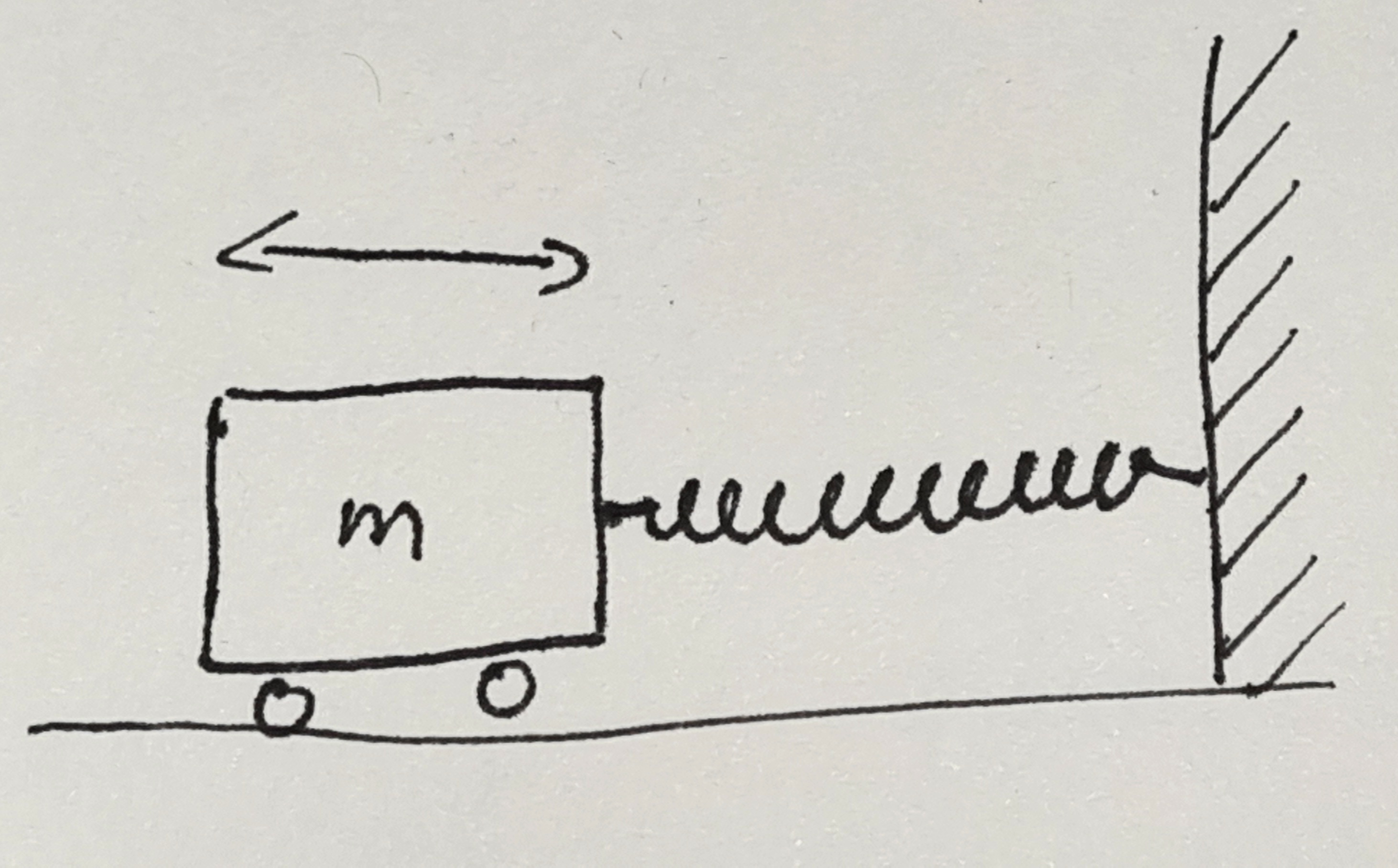
Let’s start with the most simple system that you will probably know from school. The mass on a spring is an idealized system consisting of a mass \(m\) attached to one end of a spring. The other end of the spring is held fixed. We imagine it being attached to a strong wall that will not move. The mass can only move in one direction and this motion will act to extend or contract the spring. The spring itself is assumed to be very light so that we can ignore its mass.
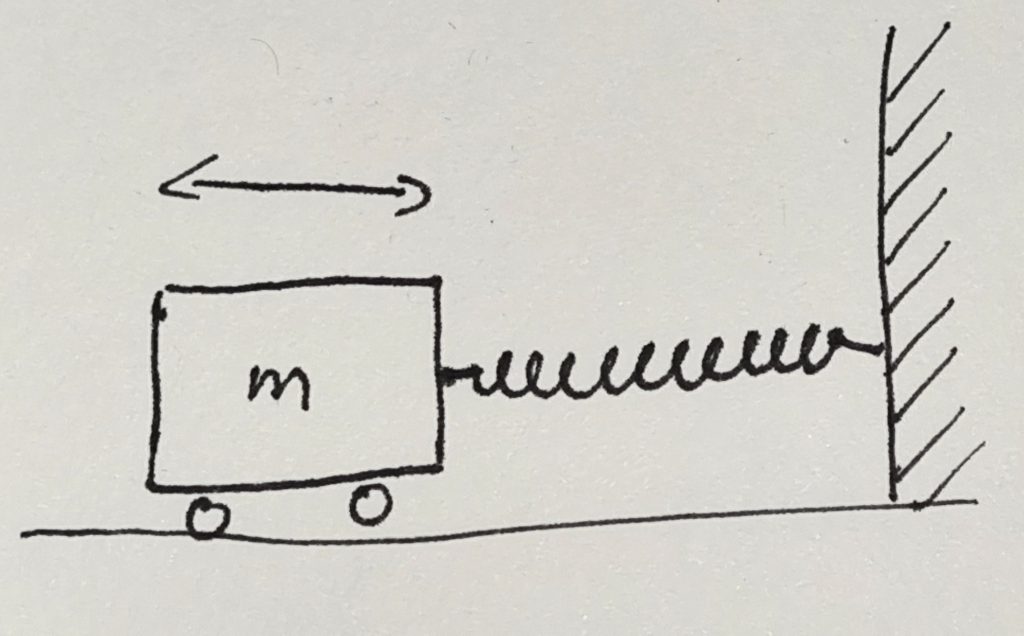
In the image, one end of the spring is attached to a wall and extends horizontally. The mass is attached to the other end and we assume that it can move without any friction. In the image, the mass has some wheels that allow it to move easily. We assume that the wheels do not create any resistance to the movement. I will come back to this assumption later.
When the system is in equilibrium, the mass will be at rest at some position along the horizontal axis. At this position, the spring does not exert any force on the mass and the mass will have no reason to move await from this equilibrium position. This is not very interesting, so let’s pull the mass away from its resting place. In what follows, I will measure the displacement, \(x\), of the mass from this equilibrium position. If we pull the mass to the right \(x\) will be positive. The spring will exert a force on the mass that will try to pull it back. The force will act towards the left, so we will assign it a negative value. A spring is designed so that the force is proportional to the displacement \(x\). The proportionality factor is called the spring constant \(k\). So we end up with a formula for the force, \[
F = -kx.
\] You can see that this formula also works if the mass is displaced to the left. In this case, \(x\) is negative and the force will be positive, pushing the mass to the right. Using the force, we can find out how the mass will move with time. The other equation that we will need for this is Newton’s law of motion, \(F = ma\) or \[
F = m \frac{d^2x}{dt^2}.
\] From these two equations we can eliminate the force and end up with \[
\frac{d^2x}{dt^2} = -\frac{k}{m}x.
\] This is a differential equation for the position \(x\). You can solve this by finding a function \(x(t)\) that, when differentiated twice, will give the same function but with a negative factor in front of it. From high school, you might remember that the \(\sin\) and \(\cos\) functions show this behavior, so let’s try it with \[
x(t) = x_0 \sin\left(\omega (t – t_0) \right).
\] Here \(x_0\), \(t_0\), and \(\omega\) are some constants that we don’t yet know. The idea is to try to keep the solution as general as possible and then see how we need to set these values to make it fit. So let’s try it out by inserting the function on both sides of our differential equation. \[
-\omega^2 x_0 \sin\left(\omega (t – t_0) \right) = -\frac{k}{m} x_0 \sin\left(\omega (t – t_0) \right).
\] Most terms in this equation cancel out and we are left with \[
\omega^2 = \frac{k}{m}.
\] This tells us that the equation of motion is satisfied whenever we choose \(\omega\) to satisfy this relation. Interestingly, the parameters \(x_0\) and \(t_0\) were canceled out which implies that we are free to choose any value for it. We could have also chosen \(\cos\) instead of \(\sin\) and ended up with the same result.
We now have a solution that depends on three parameters, \(x_0\), \(t_0\), and \(\omega\). We can do a dimensional analysis and see that \(x_0\) has units of length, \(t_0\) has units of time, and \(\omega\) is a frequency. Let’s take look at how these parameters change the behavior of the solution.
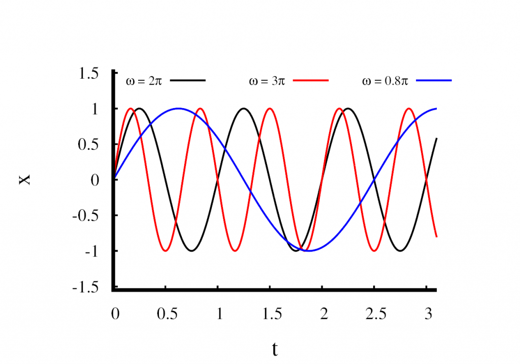
In the first figure, I have plotted three solutions in which I held \(x_0\) constant at 1m and \(t_0\) at zero. Only the parameter \(\omega\) is changed. You can see that \(\omega\) changes the speed at which the oscillations occur. A large value means that the oscillations are fast, and a small value means that the oscillations are slow. Looking at the \(\sin\) function, you can see that a full cycle finishes when the product \(\omega t\) reaches a value of \(2\pi\). This means that \(\omega\) is related to the frequency of the oscillation by \[
f = \frac{\omega}{2\pi}.
\] We call \(\omega\) the angular frequency.
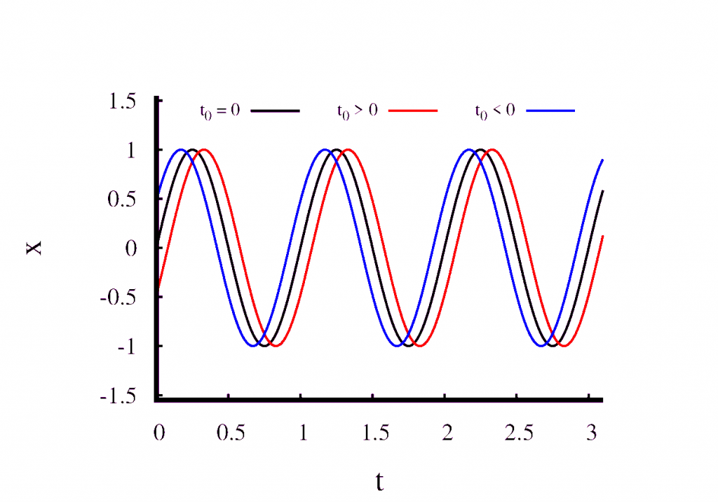
Next, have a look at what happens when we change \(t_0\) but keep all the other parameters fixed. This is shown in the second figure. You can see that \(t_0\) simply shifts the solution in time and does not modify it in any other way. We can choose \(t_0\) freely. All that this means is that we are at liberty to choose the point at which we start measuring time.
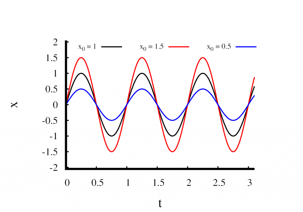
The third figure shows what happens when we modify \(x_0\) and keep all the other parameters fixed. You can clearly see that \(x_0\) changes the amplitude of the oscillation. Remember, that only the frequency \(\omega\) was fixed by the mass and the spring constant. We are free to choose \(x_0\) which means that the frequency is not influenced by our choice of \(x_0\). This leads to a very important conclusion about the harmonic oscillator.
The frequency of the oscillation is independent of its amplitude.
An energy perspective
In physics, it is often useful to look at the energy. In the spring mass system, we have two types of energy, the kinetic energy of the oscillating mass and the potential energy stored in the extended spring. We all remember the kinetic energy, \[
E_{\mathrm{kin}} = \frac{1}{2}m v^2.
\] To calculate the velocity, we have to take the derivative of the solution \(x(t)\), \[
v(t) = \omega x_0 \cos\left(\omega (t – t_0) \right).
\] The potential energy in the spring can be calculated by the work done as the spring is extended from the equilibrium length. You might remember the work to be force times distance. But in our system, the force changes with the distance. This means that the simple product has to be replaced with an integral, \[
E_{\mathrm{pot}} = \int_0^xkx\;dx = \frac{1}{2}kx^2.
\] We can take a look at the total energy over time. We know it should be constant, so let’s give it a try, \[
E_{\mathrm{tot}} = \frac{1}{2}m \omega^2 x_0^2\cos^2\left(\omega (t – t_0) \right) + \frac{1}{2}kx_0^2\sin^2\left(\omega (t – t_0) \right).
\] This can be simplified. First we can substitute \(\omega^2\) with \(k/m\). The terms in front of the trigonometric functions turn out to be the same and can be factorised, \[
E_{\mathrm{tot}} = \frac{1}{2}k x_0^2\left[\cos^2\left(\omega (t – t_0) \right) + \sin^2\left(\omega (t – t_0) \right)\right].
\] Next, Pythagoras tells us that \(\sin^2 + \cos^2 = 1\), so the bracket is just unity and we get \[
E_{\mathrm{tot}} = \frac{1}{2}k x_0^2.
\] This result confirms what we expected, the total energy is conserved and is equal to the maximum potential energy when the mass is at rest.
Another important thing to take away from this discussion is the relation between the potential energy \(E_{\mathrm{pot}} = \frac{1}{2}kx^2\) and the linear force \(F = -kx\). This relation more or less holds for any harmonic oscillator, not just the mass-and-spring system. Whenever we see a potential energy that is a parabolic function of the position, we can derive a linear force from it and we end up with a harmonic oscillator. This is why a potential of this form is also called a harmonic potential.
The oscillator in higher dimensions
The harmonic oscillator can easily be generalised to higher dimensions. Now, the displacement \(x\) is replaced by a vector \(\mathbf{r}\). The vector can be two-dimensional or three-dimensional. Then the force is also a vector and the force equation reads \[
\mathbf{F} = -k\mathbf{r}.
\] The equation states that the force always points from the position of the mass towards the origin. Just as with the one-dimensional case, the strength of the force is proportional to the distance from the origin. The force equation is relatively straightforward to grasp, but I find it slightly more instructive to look at the energy equation, \[
E_{\mathrm{pot}} = \frac{1}{2}k |\mathbf{r}|^2.
\] Let’s assume we are in three dimensions and the position vector is represented by its components \(\mathbf{r} = (x, y, z)\). We can use Pythagoras to calculate the magnitude of \(\mathbf{r}\) and end up with \[
E_{\mathrm{pot}} = \frac{1}{2}k \left(x^2 + y^2 + z^2\right).
\] Let’s write this a bit differently by expanding the bracket, \[
E_{\mathrm{pot}} = \frac{1}{2}k x^2 + \frac{1}{2}k y^2 + \frac{1}{2}k z^2.
\] You can see that this formula represents three independent harmonic oscillators. This is an important result. Imagine that the $y$ and $z$ coordinates were fixed to some value. Then the potential energy is that of a harmonic oscillator in x plus some constant offset. But it is always possible to add a constant to the potential energy because the physics only depends on potential differences. Equivalently, keeping $x$ and $z$ constant results in a harmonic oscillator in $y$.
Computational Physics: Truncation and Rounding Errors
Posted 15th October 2021 by Holger Schmitz
In a previous post, I talked about accuracy and precision in numerical calculations. Ideally one would like to perform calculations that are perfect in these two aspects. However, this is almost never possible in practical situations. The reduction of accuracy or precision is due to two numerical errors. These errors can be classified into two main groups, round-off errors and truncation errors.
Rounding Error
Round-off errors occur due to the limits of numerical precision at which numbers are stored in the computer. As I discussed here a 32-bit floating-point number for example can only store up to 7 or 8 decimal digits. Not just the final result but every intermediate result of a calculation will be rounded to this precision. In some cases, this can result in a much lower precision of the final result. One instance where round-off errors can become a problem happens when the result of a calculation is given by the difference of two large numbers.
Truncation Error
Truncation errors occur because of approximations the numerical scheme makes with respect to the underlying model. The name truncation error stems from the fact that in most schemes the underlying model is first expressed as an infinite series which is then truncated allowing it to be calculated on a computer.
Example: Approximating Pi
Let’s start with a simple task. Use a series to approximate the value of \(\pi\).
Naive summation
One of the traditional ways of calculating \(\pi\) is by using the \(\arctan\) function together with the identity \[
\arctan(1) = \frac{\pi}{4}.
\] One can expand \(\arctan\) into its Taylor series, \[
\arctan(x)
= x – \frac{x^3}{3} +\frac{x^5}{5} – \frac{x^7}{7} + \ldots
= \sum_{n=0}^\infty \frac{(-1)^n x^{2n+1}}{2n+1}.
\] The terms of the series become increasingly smaller and you could try to add up all the terms up to some maximum \(N\) in the hope that the remaining infinite sum is small and can be neglected. Inserting \(x=1\) into the sum will give you an approximation for \(\pi\), \[
\pi \approx 4\sum_{n=0}^N \frac{(-1)^n }{2n+1}.
\]
Here are e implementations for this approximation in C++, Python and JavaScript.
C++
double pi_summation_slow(int N) {
  double  sum = 0.0;
  int  sign = 1;

  for (int  i=0; i<N; ++i) {
    sum += sign/(2*i + 1.0);
    sign = -sign;
  }

  return 4*sum;
}
Python
def  pi_summation_slow(N):
  sum  =  0.0
  sign  =  1

  for  i  in  range(0,N):
    sum   =  sum  +  sign/(2*i  +  1.0)
    sign  =  -sign
    return  4*sum
JavaScript
function pi_summation_slow(N) {
  let sum = 0.0;
  let sign = 1;

  for (let i=0; i<N; ++i) {
    sum += sign/(2*i + 1.0);
    sign = -sign;
  }

  return 4*sum;
}
Let’s call this function with \(N=10\). All the results I am showing here are calculated using a Python implementation. We get a result of around 3.0418. The relative error is 0.0318 and is, of course, unacceptable. This error falls under the category of truncation errors because it is caused by not summing up enough terms of the Taylor series. Calling the function with \(N=1000\) gives us a result of 3.14059 with a relative error of \(3.183\times 10^{-4}\). The error has improved but is still far off from the possible \(10^{-14}\) to \(10^{-15}\) achievable in double-precision arithmetic. The figure below shows how the relative error decreases with the number of iterations.
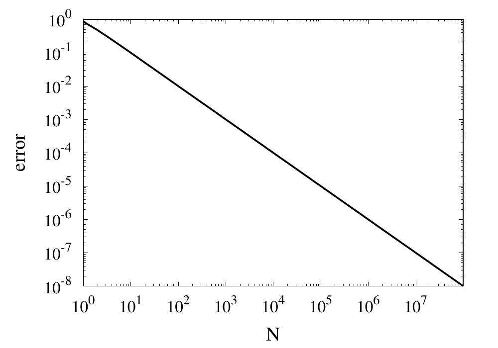
Relative error of the simple approximation of \( \pi \) depending on the number of iterations
From this curve, one h long m wl hat the error decreases with \(1/N\). If one extrapolates the curve, one finds that it would take \(10^{14}\) iterations to reach an error below \(10^{-14}\). Even if this was computationally feasible, the round-off errors of such a long sum would eventually prevent the error from being lowered to this limit.
Improvements using Machin’s formula
The technique of calculating \(\pi\) can be improved in two ways. Firstly, instead of using the Taylor series, you can use Euler’s series for the \(\arctan\) function.
\[
\arctan(x) = \sum_{n=0}^\infty \frac{2^{2n} (n!)^2}{(2n + 1)!} \frac{x^{2n + 1}}{(1 + x^2)^{n + 1}}.
\]
This series converges much more quickly than the Taylor series. The other way to improve convergence is to use trigonometric identities to come up with formulas that converge more quickly. One of the classic equations is the Machin formula for \(\pi\), first discovered by John Machin in 1706, \[
\frac{\pi}{4} = 4 \arctan \frac{1}{5} – \arctan \frac{1}{239}
\] Here are the implementations for this formula.
C++
double pi_summation_fast(int order) {
  using boost::math::factorial;
  double sum = 0.0;

  for (unsigned int n=0; n<order; ++n) {
    double f = factorial<double>(n);
    double common = pow(2.0, 2*n)*f*f/factorial<double>(2*n + 1);
    double A = pow(25./26., n+1)/pow(5., 2*n+1);
    double B = pow(239.*239. / (239.*239. + 1.), n+1)/pow(239., 2*n+1);
    sum += common*( 4*A - B );
  }

  return 4*sum;
}
Python
def pi_summation_fast(N):
  sum = 0.0

  for n in range(0,N):
    f = factorial(n)
    common = math.pow(2.0, 2*n)*f*f/factorial(2*n + 1)
    A = math.pow(25/26, n+1)/math.pow(5, 2*n+1)
    B = math.pow(239*239 / (239*239 + 1), n+1)/math.pow(239, 2*n+1)
    sum = sum + common*( 4*A - B )

  return 4*sum;
JavaScript
function pi_summation_fast(N) {
  let sum = 0.0;

  for (let n=0; n<N; ++n) {
    const f = factorial(n);
    const common = Math.pow(2.0, 2*n)*f*f/factorial(2*n + 1);
    const A = pow(25/26, n+1)/pow(5, 2*n+1);
    const B = pow(239*239 / (239*239 + 1), n+1)/pow(239, 2*n+1);
    sum += common*( 4*A - B );
  }

  return 4*sum;
}
The table below shows the computed values for \(\pi\) together with the relative error. You can see that each iteration reduces the error by more than an order of magnitude and only a few iterations are necessary to achieve machine precision accuracy.
| N | \(S_N\) | error |
|---|---|---|
| 1 | 3.060186968243409 | 0.02591223443732105 |
| 2 | 3.139082236428362 | 0.0007990906009289966 |
| 3 | 3.141509789149037 | 2.6376570705797483e-05 |
| 4 | 3.141589818359699 | 9.024817686074192e-07 |
| 5 | 3.141592554401089 | 3.157274505454055e-08 |
| 6 | 3.141592650066872 | 1.1213806035463463e-09 |
| 7 | 3.1415926534632903 | 4.0267094489200705e-11 |
| 8 | 3.1415926535852132 | 1.4578249079970333e-12 |
| 9 | 3.1415926535896266 | 5.3009244691058615e-14 |
| 10 | 3.1415926535897873 | 1.8376538159566985e-15 |
| 11 | 3.141592653589793 | 0.0 |
Example: Calculating sin(x)
Calculate the value of \(\sin(x)\) using it’s Taylor series around x=0.
The Taylor series for \(\sin(x)\) is \[
\sin x = \sum_{n=0}^\infty \frac{(-1)^n}{(2n+1)!}x^{2n+1}.
\] this series is much more well-behaved than the Taylor series for \(\arctan\) we saw above. Because of the factorial in the denominator, the individual terms of this series will converge reasonably quickly. Here are some naive implementations of this function where the infinite sum has been replaced by a sum from zero to \(N\).
C++
double taylor_sin(double x, int order)
{
  using boost::math::factorial;
  double sum = 0.0;
  int sign = 1;

  for (unsigned int n=0; n<order; ++n)
  {
    sum += sign*pow(x, 2*n + 1)/factorial<double>(2*n +1);
    sign = -sign;
  }

  return sum;
}
Python
def taylor_sin(x, N):
  sum = 0.0
  sign = 1

  for n in range(0,N):
    sum = sum + sign*math.pow(x, 2*n + 1)/factorial(2*n + 1)
    sign = -sign

  return sum
JavaScript
function taylor_sin(x, N) {
  let sum = 0.0;
  let sign = 1;

  for (let n=0; n<N; n++) {
    sum += sign*pow(x, 2*n + 1)/factorial(2*n +1);
    sign = -sign;
  }

  return sum;
}
A good test for this function is the evaluation of \(\sin(x)\) at values \(x = k\pi\), where \(k\) is an integer. We know that \(\sin(k\pi) = 0\) and the return value from the numeric function can directly be used as the absolute error of the computation. The figure below shows results for some values of \(k\) plotted against \(N\).
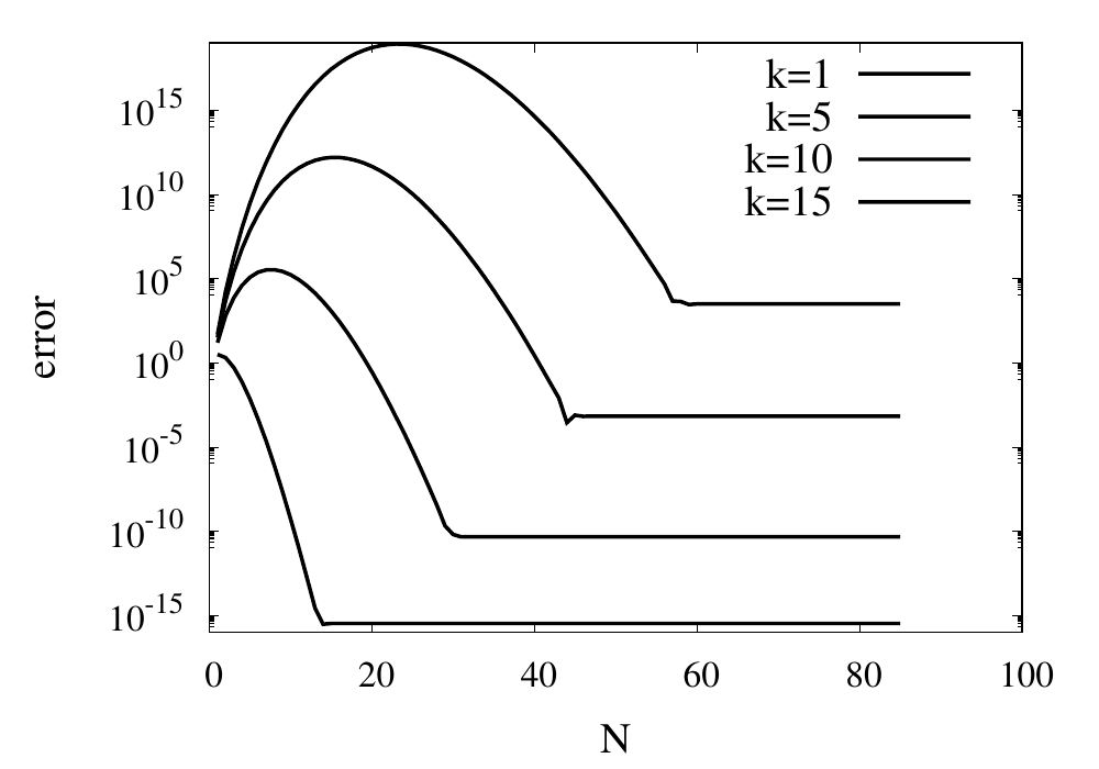
For small values of \(k\), this series converges relatively quickly. But for larger \(k\) you can see that more and more terms are needed. The error even grows first before being reduced. Just like the example above, the truncation error requires large values of \(N\) to reach a good accuracy of the result. In practice, you would not calculate the \(\sin\) function this way. Instead you would make use of known properties, such as \(\sin(2k\pi + x) = \sin(x)\) for integer \(k\), to transform the argument into a range where fast convergence is guaranteed.
However, I would like to continue my analysis of this function because it shows two more interesting pitfalls when performing long sums. First, you will notice that the curves in the figure above show dashed lines for \(N>85\). This is because the implementation I showed above will actually fail with a range error. The pow function and the factorial both start producing numbers that exceed the valid range of double floating-point numbers. The quotient of the two, on the other hand, remains well-behaved. It is, therefore, better to write the Taylor series using a recursive definition of the terms.
\[
\sin x = \sum_{n=0}^\infty a_n(x),
\] with \[
a_0 = x
\] and \[
a_{n} = -\frac{x^2}{2n(2n+1)}a_{n-1}
\]
The implementations are given again below.
C++
double taylor_sin_opt(double x, int order)
{
  double sum = x;
  double an = x;

  for (unsigned int n=1; n<order; ++n)
  {
    an = -x*x*an/(2*n*(2*n+1));
    sum += an;
  }

  return sum;
}
Python
def taylor_sin_opt(x, N):
  sum = x
  an = x

  for n in range(1,N):
    an = -x*x*an/(2*n*(2*n+1))
    sum = sum + an

  return sum
JavaScript
function taylor_sin_opt(x, N) {
  let sum = x;
  let an = x;

  for (let n=1; n<N; n++) {
    an = -x*x*an/(2*n*(2*n+1));
    sum += an;
  }

  return sum;
}
The other takeaway from the graphs of the errors is that they don’t always converge to machine accuracy. The reason for this originates from fact that the initial terms of the sum can be quite large but with opposite signs. They should cancel each other out exactly, but they don’t because of numerical round-off errors.
Spherical Blast Wave Simulation
Posted 2nd December 2020 by Holger Schmitz
Here is another animation that I made using the Vellamo fluid code. It shows two very simple simulations of spherical blast waves. The first simulation has been carried out in two dimensions. The second one shows a very similar setup but in three dimensions.
You might have seen some youtube videos on blast waves and dimensional analysis on the Sixty Symbols channel or on Numberphile. The criterion for the dimensional analysis given in those videos is true for strong blast waves. The simulation that I carried out, looks at the later stage of these waves when the energy peters out and the strong shock is replaced by a compression wave that travels at a constant velocity. You can still see some of the self-similar behaviour of the Sedov-Taylor solution during the very early stages of the explosion. But after the speed of the shock has slowed down to the sound speed, the compression wave continues to travel at the speed of sound, gradually losing its energy.
The video shows the energy density over time. The energy density includes the thermal energy as well as the kinetic energy of the gas.
For those of you who are interested in the maths and the physics, the code simulates the Euler equations of a compressible fluid. These equations are a model for an ideal adiabatic gas. For more information about the Euler equations check out my previous post.
The Euler Equations: Sod Shock Tube
Posted 30th September 2020 by Holger Schmitz
In the last post, I presented a simple derivation of the Euler fluid equations. These equations describe hydrodynamic flow in the form of three conservation equations. The three partial differential equations express the conservation of mass, the conservation of momentum, and the conservation of energy. These fundamental conservation equations are written in terms of fluxes of the densities of the conserved quantities.
In general, it is impossible to solve the Euler equations for an arbitrary problem. This means that in practice when we want to find the hydrodynamic flow in a particular situation, we have to use computers and numerical methods to calculate an approximation to the solution.
Numerical simulation codes approximate the continuous mathematical solution by storing the values of the functions at discrete points. The values are stored using a finite precision format. On most CPUs nowadays numbers will be stored as 64-bit floating-point, but for codes running on GPUs, this might be reduced to 32 bits. In addition to the discretisation in space, the equations are normally integrated using discrete steps in time. All of these factors mean that the computer only stores part of the information of the exact function.
These discretisations mean that the continuous differential equations have to be turned into a prescription how to update the discrete values from one time step to the next. For each differential equation, there are numerous ways to translate them into a numerical algorithm. Each algorithm will make different approximations and introduce different errors into the system. In general, it is impossible for a numerical algorithm to reproduce the solutions of the mathematical equations exactly. This will have implications for the physics that will be simulated with the code. Talking in terms of the Euler equations, some numerical algorithms will have problems capturing shocks, while others might smear out the solutions. Even others might cause the density to turn negative in places. Making sure that physical invariants, such as mass, momentum, and energy are conserved by the algorithm is often an important aspect when designing a numerical scheme.
The Sod Shock Tube
One of the standard tests for numerical schemes simulating the Euler equations is the Sod shock tube problem. This is a simple one-dimensional setup that is initialised with a single discontinuity in the density and energy density. It then develops a left-going rarefaction wave, a right-going shock and a somewhat slower right-going contact discontinuity. The shock tube has been proposed as a test for numerical schemes by Gary A. Sod 1978 [1]. It was then picked up by others like Philip Roe [2] or Bram van Leer [3] who made it popular. Now, it is one of the standard tests for any new solver for the Euler equations. The advantage of the Sod Shock Tube is that it has an analytical solution that can be compared against. I won’t go into the details of deriving the solution in this post. You can find a sketch of the procedure on Wikipedia.
Here, I want to present an example of the shock tube test using an algorithm by Kurganov, Noelle, and Petrova [4]. The advantage of the algorithm is that it is relatively easy to implement and that is straightforward to extend to multiple dimensions. I have implemented the algorithm in my open-source fluid code Vellamo. At the current stage, the code can only simulate the Euler equations, but it can run in 1d, 2d, or 3d. It is also parallelised so that it can run on computer clusters It uses the Schnek library to manage the computational grids, their distribution onto multiple CPUs, and the communication between the individual processes.
The video shows four simulations run with different grid resolutions. At the highest resolution of 10000 grid points, the results are more or less identical to the analytic solution. The left three panels show the density $\rho$, the momentum density $\rho v$, and the energy density $E$. These are the quantities that are actually simulated by the code. The right three panels show quantities derived from the simulation, the temperature $T$, the velocity $v$, and the pressure $p$.
Starting from the initial discontinuity at $x=0.5$ you can see a rarefaction wave moving to the left. The density $\rho$ has a negative slope whereas the momentum density $\rho v$ increases in this region. In the plot of the velocity, you can see a linear slope, indicating that the fluid is being accelerated by the pressure gradient. The expansion of the fluid causes cooling and the temperature $T$ decreases inside the rarefaction wave.
While the rarefaction wave moves left, a shock wave develops on the very right moving into the undisturbed fluid. All six graphs show a discontinuity at the shock. The density jumps $\rho$ as the fluid is compressed and the velocity $v$ rises from 0 to almost 1 as the expanding fluid pushes into the undisturbed background. The compression also causes a sudden increase in pressure $p$ and temperature $T$.
To the left of the shock wave, you can observe another discontinuity in some but not all quantities. This is what is known as a contact discontinuity. To the left of the discontinuity, the density $\rho$ is high and the temperature $T$ is low whereas to the right density $\rho$ is low and the temperature $T$ is high. Both effects cancel each other when calculating the pressure which is the same on both sides of the discontinuity. And because there is no pressure difference, the fluid is not accelerated either, and the velocity $v$ is the same on both sides as well.
If you look at the plots of the velocity $v$ and the pressure $p$ you can’t make out where the contact discontinuity is. In a way, this is quite extraordinary because these two quantities are calculated from the density $\rho$, the momentum density $\rho v$ and the energy density $E$. All of these quantities have jumps at the location of the contact discontinuity. The level to which the derived quantities stay constant across the discontinuity is an indicator of the quality of the numerical scheme.
The simulations with lower grid resolutions show how the scheme degrades. At 1000 grid points, the results are still very close to the exact solution. The discontinuities are slightly smeared out. If you look closely at the temperature profile, you can see a slight overshoot on the high-temperature side of the contact discontinuity. At 100 grid points, the discontinuities are more smeared out. The overshoot in the temperature is more pronounced and now you can also see an overshoot at the right end of the rarefaction wave. This overshoot is present in most quantities.
As a rule of thumb, a numerical scheme for hyperbolic differential equations has to balance accuracy against numerical diffusion. In regions where the solution is well behaved, high order schemes will provide very good accuracy. Near discontinuities, however, a high order scheme will tend to produce artificial oscillations. These artefacts can create non-physical behaviour when, for instance, the numerical solution predicts a negative density or temperature. A good scheme detects the conditions where the high order algorithm fails and falls back to a lower order in those regions. This will naturally introduce some numerical diffusion into the system.
At the lowest resolution with 50 grid points, the discontinuities are even more spread out. Nonetheless, at later times in the simulation, all discontinuities can be seen and the speed at which these discontinuities move compares well with the exact result.
I hope you have enjoyed this article. If you have any questions, suggestions, or corrections please leave a comment below. If you are interested in contributing to Vellamo or Schnek feel free to contact me via Facebook or LinkedIn.
[1] Sod, G.A., 1978. A survey of several finite difference methods for systems of nonlinear hyperbolic conservation laws. Journal of computational physics, 27(1), pp.1-31.
[2] Roe, P.L., 1981. Approximate Riemann solvers, parameter vectors, and difference schemes. Journal of computational physics, 43(2), pp.357-372.
[3] Van Leer, B., 1979. Towards the ultimate conservative difference scheme. V. A second-order sequel to Godunov’s method. Journal of Computational Physics, 32(1), pp.101-136.
[4] Kurganov, A., Noelle, S. and Petrova, G., 2001. Semidiscrete central-upwind schemes for hyperbolic conservation laws and Hamilton–Jacobi equations. SIAM Journal on Scientific Computing, 23(3), pp.707-740.
The Euler Equations
Posted 3rd September 2020 by Holger Schmitz
Leonhard Euler was not only brilliant but also a very productive mathematician. In this post, I want to talk about one of the many things named after the Swiss genius, the Euler equations. These should not be confused with the Euler identity, that famous relation involving $e$, $i$, and $\pi$. No, the Euler equations are a set of partial differential equations that can be used to describe fluid flow. They are related to the Navier-Stokes equations which are at the heart of one of the unsolved Millenium Problems of the Clay Mathematics Institute.
In this short series of posts, I want to present a phenomenological derivation of the equations in one dimension. This derivation is not mathematically rigorous, but will hopefully give you an understanding of the physics that the equations are describing.
Conservation Laws
One way to understand the Euler equations is to write them in the form of conservation laws. Each equation represents a basic conservation law of physics. A central concept in these conservation equation is flux. In a 1d description, the flux of a quantity is a measure for the amount of that quantity that passes through a point. In 2d it’s the amount passing through a line and in 3d through a surface, but let’s stick to 1d during this article.
Take some quantity $N$. To make it concrete, imagine something like the total mass or number of atoms in a volume. I am using the word volume loosely. In 1d a volume is the same as an interval. Let’s call the flux of this quantity $F$. The flux can be different at different locations, so $F$ is a function of position $x$, in other words, the flux is $F(x)$.
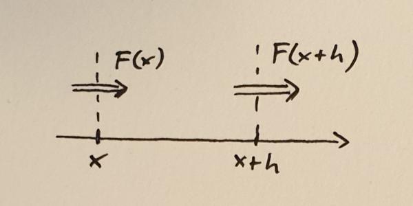
Flux into and out of a small volume between $x$ and $x+h$
Next, consider a small volume between $x$ and $x+h$. Here $h$ is the width of the volume and you should think of it as a small quantity. The rate of change of the quantity $N$ within this volume is determined by the difference between the flux into the volume and the flux out of the volume. If we take positive flux to mean that the quantity (mass, number of atoms, stuff) is moving to the right, then we can write down the following equation.
$$\frac{dN}{dt} = F(x) – F(x+h)$$
Here the left-hand side of the equation represents the rate of change of $N$. I have not written it here but, of course, $N$ depends on the position $x$ as well as the with of the volume $h$. The next step to turn this into a conservation equation is to divide both sides by $h$.
$$\frac{d}{dt}\left(\frac{N}{h}\right) = -\frac{F(x+h) – F(x)}{h}$$
If you remember your calculus lessons, you might already see where this is going. We now make $h$ smaller and smaller and look at the limit when $h \to 0$. The right hand side of the equation will give us the derivative of $F$,
$$\lim_{h \to 0} \frac{F(x+h) – F(x)}{h} = \frac{dF}{dx}$$
The amount of stuff $N$ in the volume will shrink and shrink as $h$ decreases, but because we are dividing by $h$ the ratio $N/h$ will converge to a sensible value. Let’s call this value $n$,
$$n = \lim_{h \to 0}\frac{N}{h}.$$
The quantity $n$ is called the density of $N$. Now the conservation law is simply written as
$$\frac{\partial n}{\partial t} = -\frac{\partial F}{\partial x}.$$
This equation expresses the change of the density of the conserved quantity through the derivative of the flux of that quantity.
The Equations
Now that the basic form of the conservation equations is established, let’s look at some quantities that are conserved and that can be used to express fluid flow. The first conservation law to look at is the conservation of mass. Note again that the conservation equation is written in terms of the density of the conserved quantity. The mass density is the mass contained in a small volume divided by that volume. It is often abbreviated by the Greek letter $\rho$ (rho).
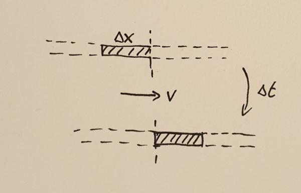
Matter crossing a point during the time interval $\Delta t$
In order to find out what the mass flux is, consider the fluid moving with velocity $v$ through some point. During a small time interval, $\Delta t$ the fluid will move by a small distance $\Delta x$. All the mass $M$ contained in the interval of width $\Delta x$ will cross the point. This mass can be calculated to be
$$M = \rho \Delta x.$$
The flux is the amount of mass crossing the point divided by the time it took the mass to cross that point, $F_{\rho} = M / \Delta t$. In other words,
$$F_{\rho} = \rho \frac{\Delta x}{\Delta t} = \rho v.$$
This now lets us write the mass conservation equation,
$$\frac{\partial \rho}{\partial t} = -\frac{\partial }{\partial x}(\rho v).$$
What does this equation mean? Let me explain this with two examples. First, imagine a constant flow velocity $v$ but an increasing density profile $\rho(x)$. At any given point the density will decrease because the density profile will constantly move towards the right without changing shape. The lower density that was previously located at somewhat left of $x$ will move to the point $x$ thus decreasing the density there.
For the other example, imagine that the density is constant but the velocity has an increasing profile. Matter to the right will flow faster than matter to the left. This will also decrease the density over time because the existing mass is constantly thinned out.
The next conservation equation expresses the conservation of momentum. Momentum is mass times velocity and therefore momentum density is mass density times velocity, $\rho v$. In the mass conservation equation, you could see that the flux consists only of the conserved density multiplied with the velocity. This is called the convective term and this term is present in all Euler equations. However, the momentum can also change through a force. Without external forces, the only force onto each fluid element is through the pressure $p$. The momentum conservation equation can be written as
$$\frac{\partial }{\partial t}(\rho v) = -\frac{\partial }{\partial x}(\rho v^2 + p).$$
The last conservation equation is the conservation of energy, expressed by the energy density $e$,
$$\frac{\partial e}{\partial t} = -\frac{\partial }{\partial x}(e v + p v).$$
The first term is again the convective term expressing the transport of energy contained in the fluid as the fluid moves. The second term is the work done by the pressure force. Note that the energy density $e$ contains the internal (heat) energy as well as the kinetic energy of the fluid moving as a whole.
Finally, we need to close the set of equations by defining what the pressure $p$ is. This closure depends on the type of fluid you want to model. For an ideal gas, the pressure is related to the other variables through
$$p = (\gamma – 1)\left(E – \frac{\rho v^2}{2}\right).$$
Here $\gamma$ is the adiabatic gas index. The second bracket on the right-hand side is the internal energy, expressed as the total energy minus the kinetic energy of the flow.
Putting it All Together
In summary, the Euler equations are conservation equations for the mass, momentum, and energy in the system. In 1d, they can be written as
$$\begin{eqnarray}
\frac{\partial }{\partial t}\rho &=& -\frac{\partial }{\partial x}(\rho v) \\
\frac{\partial }{\partial t}(\rho v) &=& -\frac{\partial }{\partial x}(\rho v^2 + p) \\
\frac{\partial }{\partial t}e &=& -\frac{\partial }{\partial x}(e v + p v)
\end{eqnarray}
$$
In higher dimensions, the derivative with respect to $x$ is replaced by the divergence operator $\nabla$.
$$\begin{eqnarray}
\frac{\partial }{\partial t}\rho &=& -\nabla(\rho \mathbf{v}) \\
\frac{\partial }{\partial t}(\rho v) &=& -\nabla(\rho \mathbf{v}\otimes\mathbf{v} + p\mathbf{I}) \\
\frac{\partial }{\partial t}e &=& -\nabla(e \mathbf{v} + p \mathbf{v})
\end{eqnarray}
$$
The $\otimes$ symbol denotes the outer product of the velocity vectors. It multiplies two vectors to produce a matrix. I will not go into the definition of the outer product here. You can read more on Wikipedia. The symbol $\mathbf{I}$ is the identity matrix.
Summary
The Euler equations are a set of partial differential equations describing fluid flow. When Euler published a simpler version of these equations, they were one of the earliest examples of partial differential equations. Today, the Euler equations and their generalisations, including the Navier-Stokes equations provide the basis for understanding fluid behaviour, turbulence, and the weather.
The Euler equations are difficult to solve and only some special solutions can be written down on paper. For the general case, we need computers to give us answers. In the next post, I will show the results of some simulations I have created with my freely available fluid code Vellamo.