Computational Physics Basics: Polynomial Interpolation
Posted 19th April 2023 by Holger Schmitz
The piecewise constant interpolation and the linear interpolation seen in the previous post can be understood as special cases of a more general interpolation method. Piecewise constant interpolation constructs a polynomial of order 0 that passes through a single point. Linear interpolation constructs a polynomial of order 1 that passes through 2 points. We can generalise this idea to construct a polynomial of order \(n-1\) that passes through \(n\) points, where \(n\) is 1 or greater. The idea is that a higher-order polynomial will be better at approximating the exact function. We will see later that this idea is only justified in certain cases and that higher-order interpolations can actually increase the error when not applied with care.
Existence
The first question that arises is the following. Given a set of \(n\) points, is there always a polynomial of order \(n-1\) that passes through these points, or are there multiple polynomials with that quality? The first question can be answered simply by constructing a polynomial. The simplest way to do this is to construct the Lagrange Polynomial. Assume we are given a set of points, \[
(x_1, y_1), (x_2, y_2) \ldots (x_n, y_n),
\] where all the \(x\)’s are different, i.e. \(x_i \ne x_j\) if \(i \ne j\). Then we observe that the fraction \[
\frac{x – x_j}{x_i – x_j}
\] is zero when \(x = x_j\) and one when \(x = x_i\). Next, let’s choose an index \(i\) and multiply these fractions together for all \(j\) that are different to \(i\), \[
a_i(x) = \frac{x – x_1}{x_i – x_1}\times \ldots\times\frac{x – x_{i-1}}{x_i – x_{i-1}}
\frac{x – x_{i+1}}{x_i – x_{i+1}}\times \ldots\times\frac{x – x_n}{x_i – x_n}.
\] This product can be written a bit more concisely as \[
a_i(x) = \prod_{\stackrel{j=1}{j\ne i}}^n \frac{x – x_j}{x_i – x_j}.
\] You can see that the \(a_i\) are polynomials of order \(n-1\). Now, if \(x = x_i\) all the factors in the product are 1 which means that \(a_i(x_i) = 1\). On the other hand, if \(x\) is any of the other \(x_j\) then one of the factors will be zero and \(a_i(x_j) = 0\) for any \(j \ne i\). Thus, if we take the product \(a_i(x) y_i\) we have a polynomial that passes through the point \((x_i, y_i)\) but is zero at all the other \(x_j\). The final step is to add up all these separate polynomials to construct the Lagrange Polynomial, \[
p(x) = a_1(x)y_1 + \ldots a_n(x)y_n = \sum_{i=1}^n a_i(x)y_i.
\] By construction, this polynomial of order \(n-1\) passes through all the points \((x_i, y_i)\).
Uniqueness
The next question is if there are other polynomials that pass through all the points, or is the Lagrange Polynomial the only one? The answer is that there is exactly one polynomial of order \(n\) that passes through \(n\) given points. This follows directly from the fundamental theorem of algebra. Imagine we have two order \(n-1\) polynomials, \(p_1\) and \(p_2\), that both pass through our \(n\) points. Then the difference, \[
d(x) = p_1(x) – p_2(x),
\] will also be an order \(n-1\) degree polynomial. But \(d\) also has \(n\) roots because \(d(x_i) = 0\) for all \(i\). But the fundamental theorem of algebra asserts that a polynomial of degree \(n\) can have at most \(n\) real roots unless it is identically zero. In our case \(d\) is of order \(n-1\) and should only have \(n-1\) roots. The fact that it has \(n\) roots means that \(d \equiv 0\). This in turn means that \(p_1 = p_2\) must be the same polynomial.
Approximation Error and Runge’s Phenomenon
One would expect that the higher order interpolations will reduce the error of the approximation and that it would always be best to use the highest possible order. One can find the upper bounds of the error using a similar approach that I used in the previous post on linear interpolation. I will not show the proof here, because it is a bit more tedious and doesn’t give any deeper insights. Given a function \(f(x)\) over an interval \(a\le x \le b\) and sampled at \(n+1\) equidistant points \(x_i = a + hi\), with \(i=0, \ldots , n+1\) and \(h = (b-a)/n\), then the order \(n\) Lagrange polynomial that passes through the points will have an error given by the following formula. \[
\left|R_n(x)\right| \leq \frac{h^{n+1}}{4(n+1)} \left|f^{(n+1)}(x)\right|_{\mathrm{max}}
\] Here \(f^{(n+1)}(x)\) means the \((n+1)\)th derivative of the the function \(f\) and the \(\left|.\right|_{\mathrm{max}}\) means the maximum value over the interval between \(a\) and \(b\). As expected, the error is proportional to \(h^{n+1}\). At first sight, this implies that increasing the number of points, and thus reducing \(h\) while at the same time increasing \(n\) will reduce the error. The problem arises, however, for some functions \(f\) whose \(n\)-th derivatives grow with \(n\). The example put forward by Runge is the function \[
f(x) = \frac{1}{1+25x^2}.
\]
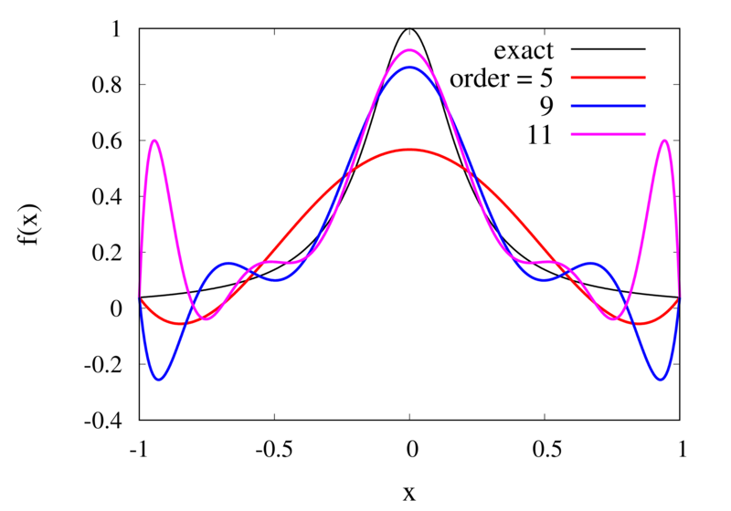
Interpolation of Runge’s function using higher-order polynomials.
The figure above shows the Lagrange polynomials approximating Runge’s function over the interval from -1 to 1 for some orders. You can immediately see that the approximations tend to improve in the central part as the order increases. But near the outermost points, the Lagrange polynomials oscillate more and more wildly as the number of points is increased. The conclusion is that one has to be careful when increasing the interpolation order because spurious oscillations may actually degrade the approximation.
Piecewise Polynomial Interpolation
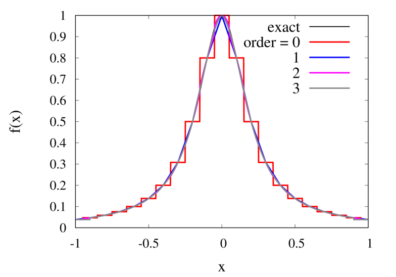
Does this mean we are stuck and that moving to higher orders is generally bad? No, we can make use of higher-order interpolations but we have to be careful. Note, that the polynomial interpolation does get better in the central region when we decrease the spacing between the points. When we used piecewise linear of constant interpolation, we chose the points that were used for the interpolation based on where we wanted to interpolate the function. In the same way, we can choose the points through which we construct the polynomial so that they are always symmetric around \(x\). Some plots of this piecewise polynomial interpolation are shown in the plot below.
Piecewise Lagrange interpolation with 20 points for orders 0, 1, 2, and 3.
Let’s analyse the error of these approximations. Using an array with \(N\) points on Runge’s function equally spaced between -2 and 2. \(N\) was varied between 10 and 10,000. For each \(N\), the centred polynomial interpolation of orders 0, 1, 2, and 3 was created. Finally, the maximum error of the interpolation and the exact function over the interval -1 and 1 are determined.
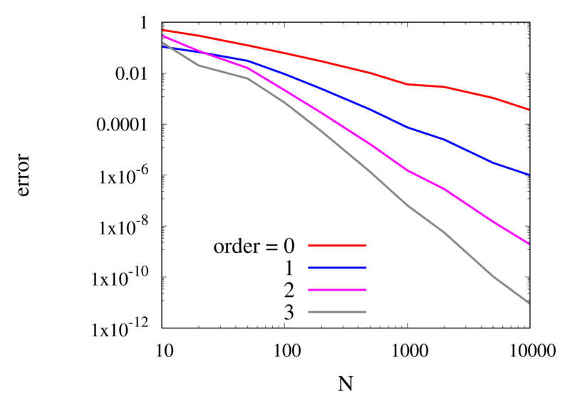
Scaling of the maximum error of the Lagrange interpolation with the number of points for increasing order.
The plot above shows the double-logarithmic dependence of the error against the number of points for each order interpolation. The slope of each curve corresponds to the order of the interpolation. For the piecewise constant interpolation, an increase in the number of points by 3 orders of magnitude also corresponds to a reduction of the error by three orders of magnitude. This indicates that the error is first order in this case. For the highest order interpolation and 10,000 points, the error reaches the rounding error of double precision.
Discontinuities and Differentiability
As seen in the previous section, for many cases the piecewise polynomial interpolation can provide a good approximation to the underlying function. However, in some cases, we need to use the first or second derivative of our interpolation. In these cases, the Lagrange formula is not ideal. To see this, the following image shows the interpolation error, again for Runge’s function, using order 2 and 3 polynomials and 20 points.
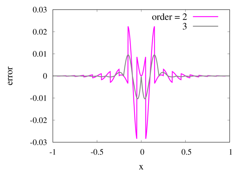
Error in the Lagrange interpolation of Runge’s function for orders 2 and 3.
One can see that the error in the order 2 approximation has discontinuities and the error in the order 3 approximation has discontinuities of the derivative. For odd-order interpolations, the points that are used for the interpolation change when \(x\) moves from an interval \([x_{i-1},x_i]\) to an interval \([x_i, x_{i+1}]\). Because both interpolations are the same at the point \(x_i\) itself, the interpolation is continuous but the derivative, in general, is not. For even-order interpolations, the stencil changes halfway between the points, which means that the function is discontinuous there. I will address this problem in a future post.
Computational Physics Basics: Piecewise and Linear Interpolation
Posted 24th February 2022 by Holger Schmitz
One of the main challenges of computational physics is the problem of representing continuous functions in time and space using the finite resources supplied by the computer. A mathematical function of one or more continuous variables naturally has an infinite number of degrees of freedom. These need to be reduced in some manner to be stored in the finite memory available. Maybe the most intuitive way of achieving this goal is by sampling the function at a discrete set of points. We can store the values of the function as a lookup table in memory. It is then straightforward to retrieve the values at the sampling points. However, in many cases, the function values at arbitrary points between the sampling points are needed. It is then necessary to interpolate the function from the given data.
Apart from the interpolation problem, the pointwise discretisation of a function raises another problem. In some cases, the domain over which the function is required is not known in advance. The computer only stores a finite set of points and these points can cover only a finite domain. Extrapolation can be used if the asymptotic behaviour of the function is known. Also, clever spacing of the sample points or transformations of the domain can aid in improving the accuracy of the interpolated and extrapolated function values.
In this post, I will be talking about the interpolation of functions in a single variable. Functions with a higher-dimensional domain will be the subject of a future post.
Functions of a single variable
A function of a single variable, \(f(x)\), can be discretised by specifying the function values at sample locations \(x_i\), where \(i=1 \ldots N\). For now, we don’t require these locations to be evenly spaced but I will assume that they are sorted. This means that \(x_i < x_{i+1}\) for all \(i\). Let’s define the function values, \(y_i\), as \[
y_i = f(x_i).
\] The intuitive idea behind this discretisation is that the function values can be thought of as a number of measurements. The \(y_i\) provide incomplete information about the function. To reconstruct the function over a continuous domain an interpolation scheme needs to be specified.
Piecewise Constant Interpolation
The simplest interpolation scheme is the piecewise constant interpolation, also known as the nearest neighbour interpolation. Given a location \(x\) the goal is to find a value of \(i\) such that \[
|x-x_i| \le |x-x_j| \quad \text{for all} \quad j\ne i.
\] In other words, \(x_i\) is the sample location that is closest to \(x\) when compared to the other sample locations. Then, define the interpolation function \(p_0\) as \[
p_0(x) = f(x_i)
\] with \(x_i\) as defined above. The value of the interpolation is simply the value of the sampled function at the sample point closest to \(x\).
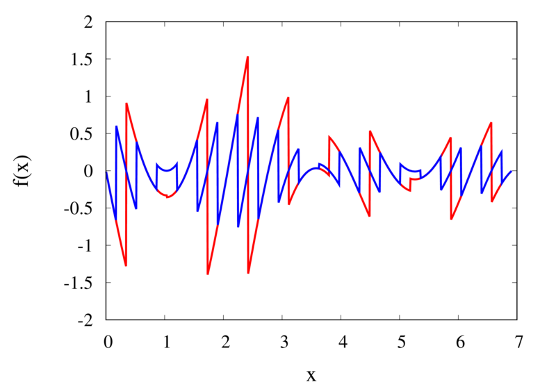
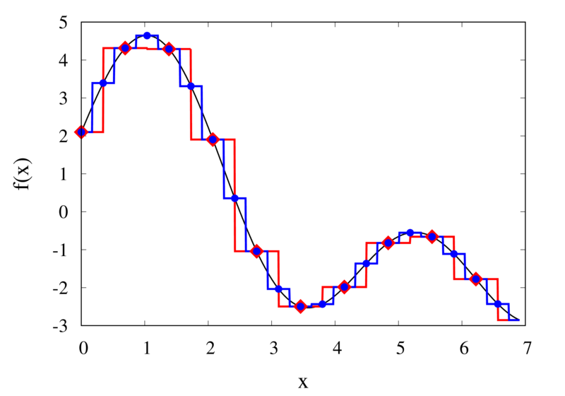
Piecewise constant interpolation of a function (left) and the error (right)
The left plot in the figure above shows some smooth function in black and a number of sample points. The case where 10 sample points are taken is shown by the diamonds and the case for 20 sample points is shown by the circles. Also shown are the nearest neighbour interpolations for these two cases. The red curve shows the interpolated function for 10 samples and the blue curve is for the case of 20 samples. The right plot in the figure shows the difference between the original function and the interpolations. Again, the red curve is for the case of 10 samples and the blue curve is for the case of 20 samples. We can see that the piecewise constant interpolation is crude and the errors are quite large.
As expected, the error is smaller when the number of samples is increased. To analyse exactly how big the error is, consider the residual for the zero-order interpolation \[
R_0(x) = f(x) – p_0(x) = f(x) – f(x_i).
\] The first step to analyse the magnitude of the residual is to perform a Taylor expansion of the residual around the point \(x_i\). We only need the zero order term. Using Taylor’s Theorem and the Cauchy form of the remainder, one can write \[
R_0(x) = \left[ f(x_i) + f'(\xi_c)(x – x_i)\right] – f(x_i).
\] The term in the brackets is the Taylor expansion of \(f(x)\), and \(\xi_c\) is some value that lies between \(x_i\) and \(x\) and depends on the value of \(x\). Let’s define the distance between two samples with \(h=x_{i+1}-x_i\). Assume for the moment that all samples are equidistant. It is not difficult to generalise the arguments for the case when the support points are not equidistant. This means, the maximum value of \(x – x_i\) is half of the distance between two samples, i.e. \[
x – x_i \le \frac{h}{2}.
\] It os also clear that \(f'(\xi_c) \le |f'(x)|_{\mathrm{max}}\), where the maximum is over the interval \(|x-x_i| \le h/2\). The final result for an estimate of the residual error is \[
|R_0(x)| \le\frac{h}{2} |f'(x)|_{\mathrm{max}}
\]
Linear Interpolation
As we saw above, the piecewise interpolation is easy to implement but the errors can be quite large. Most of the time, linear interpolation is a much better alternative. For functions of a single argument, as we are considering here, the computational expense is not much higher than the piecewise interpolation but the resulting accuracy is much better. Given a location \(x\), first find \(i\) such that \[
x_i \le x < x_{i+1}.
\] Then the linear interpolation function \(p_1\) can be defined as \[
p_1(x) = \frac{x_{i+1} – x}{x_{i+1} – x_i} f(x_i)
+ \frac{x – x_i}{x_{i+1} – x_i} f(x_{i+1}).
\] The function \(p_1\) at a point \(x\) can be viewed as a weighted average of the original function values at the neighbouring points \(x_i\) and \(x_{i+1}\). It can be easily seen that \(p(x_i) = f(x_i)\) for all \(i\), i.e. the interpolation goes through the sample points exactly.
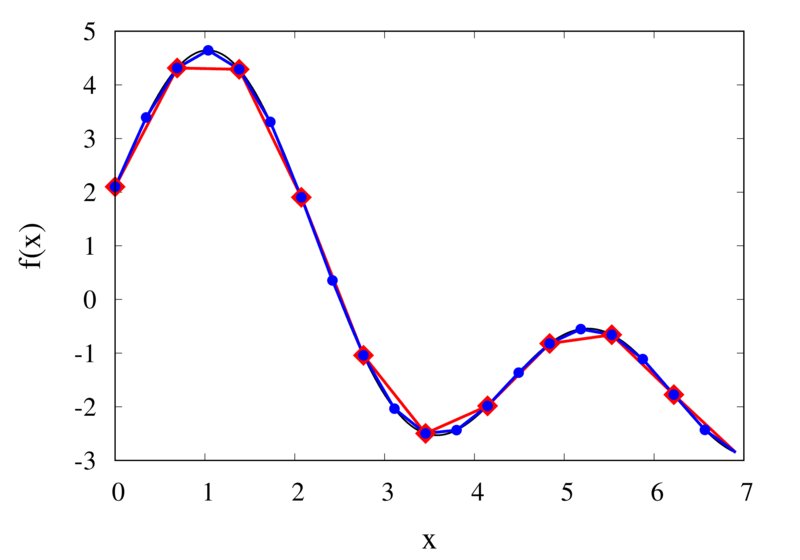
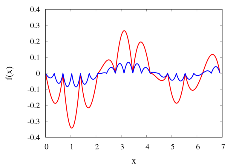
Linear interpolation of a function (left) and the error (right)
The left plot in the figure above shows the same function \(f(x)\) as the figure in the previous section but now together with the linear interpolations for 10 samples (red curve) and 20 samples (blue curve). One can immediately see that the linear interpolation resembles the original function much more closely. The right plot shows the error for the two interpolations. The error is much smaller when compared to the error for the piecewise interpolation. For the 10 sample interpolation, the maximum absolute error of the linear interpolation is about 0.45 compared to a value of over 1.5 for the nearest neighbour interpolation. What’s more, going from 10 to 20 samples improves the error substantially.
One can again try to quantify the error of the linear approximation using Taylor’s Theorem. The first step is to use the Mean Value Theorem that states that there is a point \(x_c\) between \(x_i\) and \(x_{i+1}\) that satisfies \[
f'(x_c) = \frac{ f(x_{i+1}) – f(x_i) }{ x_{i+1} – x_i }.
\] Consider now the error of the linear approximation, \[
R_1(x) = f(x) – p_1(x) = f(x) – \left[\frac{x_{i+1} – x}{x_{i+1} – x_i} f(x_i)
+ \frac{x – x_i}{x_{i+1} – x_i} f(x_{i+1})\right].
\] The derivative of the error is \[
R’_1(x) = f'(x) – \frac{ f(x_{i+1}) – f(x_i) }{ x_{i+1} – x_i }.
\] The Mean Value Theorem implies that the derivative of the error at \(x_c\) is zero and the error is at its maximum at that point. In other words, to estimate the maximum error, we only need to find an upper bound of \(|R(x_c)|\).
We now perform a Taylor expansion of the error around \(x_c\). Using again the Cauchy form of the remainder, we find \[
R(x) = R(x_c) + xR'(x_c) + \frac{1}{2}R’^\prime(\xi_c)(x-\xi_c)(x-x_c).
\] The second term on the right hand side is zero by construction, and we have \[
R(x) = R(x_c) + \frac{1}{2}R’^\prime(\xi_c)(x-\xi_c)(x-x_c).
\] Let \(h\) again denote the distance between the two points, \(h=x_{i+1} – x_i\). We assume that \(x_c – x_i < h/2\) and use the equation above to calculate \(R(x_i)\) which we know is zero. If \(x_c\) was closer to \(x_{i+1}\) we would have to calculate \(R(x_{i+1})\) but otherwise the argument would remain the same. So, \[
R(x_i) = 0 = R(x_c) + \frac{1}{2}R’^\prime(\xi_c)(x_i-\xi_c)(x_i-x_c)
\] from which we get \[
|R(x_c)| = \frac{1}{2}|R’^\prime(\xi_c)(x_i-\xi_c)(x_i-x_c)|.
\] To get an upper estimate of the remainder that does not depend on \(x_c\) or \(\xi_c\) we can use the fact that both \(x_i-\xi_c \le h/2\) and \(x_i-x_c \le h/2\). We also know that \(|R(x)| \le |R(x_c)|\) over the interval from \(x_i\) to \(x_{i+1}\) and \(|R’^\prime(\xi_c)| = |f’^\prime(\xi_c)| \le |f’^\prime(x)|_{\mathrm{max}}\). Given all this, we end up with \[
|R(x)| \le \frac{h^2}{8}|f’^\prime(x)|_{\mathrm{max}}.
\]
The error of the linear interpolation scales with \(h^2\), in contrast to \(h\) for the piecewise constant interpolation. This means that increasing the number of samples gives us much more profit in terms of accuracy. Linear interpolation is often the method of choice because of its relative simplicity combined with reasonable accuracy. In a future post, I will be looking at higher-order interpolations. These higher-order schemes will scale even better with the number of samples but this improvement comes at a cost. We will see that the price to be paid is not only a higher computational expense but also the introduction of spurious oscillations that are not present in the original data.
Computational Physics: Truncation and Rounding Errors
Posted 15th October 2021 by Holger Schmitz
In a previous post, I talked about accuracy and precision in numerical calculations. Ideally one would like to perform calculations that are perfect in these two aspects. However, this is almost never possible in practical situations. The reduction of accuracy or precision is due to two numerical errors. These errors can be classified into two main groups, round-off errors and truncation errors.
Rounding Error
Round-off errors occur due to the limits of numerical precision at which numbers are stored in the computer. As I discussed here a 32-bit floating-point number for example can only store up to 7 or 8 decimal digits. Not just the final result but every intermediate result of a calculation will be rounded to this precision. In some cases, this can result in a much lower precision of the final result. One instance where round-off errors can become a problem happens when the result of a calculation is given by the difference of two large numbers.
Truncation Error
Truncation errors occur because of approximations the numerical scheme makes with respect to the underlying model. The name truncation error stems from the fact that in most schemes the underlying model is first expressed as an infinite series which is then truncated allowing it to be calculated on a computer.
Example: Approximating Pi
Let’s start with a simple task. Use a series to approximate the value of \(\pi\).
Naive summation
One of the traditional ways of calculating \(\pi\) is by using the \(\arctan\) function together with the identity \[
\arctan(1) = \frac{\pi}{4}.
\] One can expand \(\arctan\) into its Taylor series, \[
\arctan(x)
= x – \frac{x^3}{3} +\frac{x^5}{5} – \frac{x^7}{7} + \ldots
= \sum_{n=0}^\infty \frac{(-1)^n x^{2n+1}}{2n+1}.
\] The terms of the series become increasingly smaller and you could try to add up all the terms up to some maximum \(N\) in the hope that the remaining infinite sum is small and can be neglected. Inserting \(x=1\) into the sum will give you an approximation for \(\pi\), \[
\pi \approx 4\sum_{n=0}^N \frac{(-1)^n }{2n+1}.
\]
Here are e implementations for this approximation in C++, Python and JavaScript.
C++
double pi_summation_slow(int N) {
  double  sum = 0.0;
  int  sign = 1;

  for (int  i=0; i<N; ++i) {
    sum += sign/(2*i + 1.0);
    sign = -sign;
  }

  return 4*sum;
}
Python
def  pi_summation_slow(N):
  sum  =  0.0
  sign  =  1

  for  i  in  range(0,N):
    sum   =  sum  +  sign/(2*i  +  1.0)
    sign  =  -sign
    return  4*sum
JavaScript
function pi_summation_slow(N) {
  let sum = 0.0;
  let sign = 1;

  for (let i=0; i<N; ++i) {
    sum += sign/(2*i + 1.0);
    sign = -sign;
  }

  return 4*sum;
}
Let’s call this function with \(N=10\). All the results I am showing here are calculated using a Python implementation. We get a result of around 3.0418. The relative error is 0.0318 and is, of course, unacceptable. This error falls under the category of truncation errors because it is caused by not summing up enough terms of the Taylor series. Calling the function with \(N=1000\) gives us a result of 3.14059 with a relative error of \(3.183\times 10^{-4}\). The error has improved but is still far off from the possible \(10^{-14}\) to \(10^{-15}\) achievable in double-precision arithmetic. The figure below shows how the relative error decreases with the number of iterations.
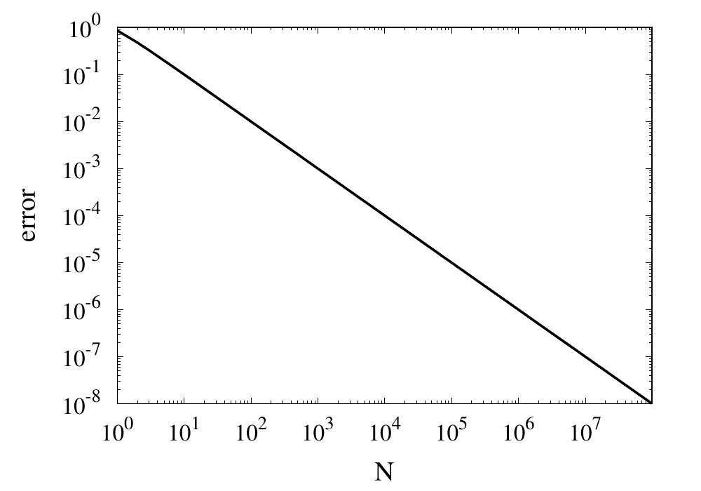
Relative error of the simple approximation of \( \pi \) depending on the number of iterations
From this curve, one h long m wl hat the error decreases with \(1/N\). If one extrapolates the curve, one finds that it would take \(10^{14}\) iterations to reach an error below \(10^{-14}\). Even if this was computationally feasible, the round-off errors of such a long sum would eventually prevent the error from being lowered to this limit.
Improvements using Machin’s formula
The technique of calculating \(\pi\) can be improved in two ways. Firstly, instead of using the Taylor series, you can use Euler’s series for the \(\arctan\) function.
\[
\arctan(x) = \sum_{n=0}^\infty \frac{2^{2n} (n!)^2}{(2n + 1)!} \frac{x^{2n + 1}}{(1 + x^2)^{n + 1}}.
\]
This series converges much more quickly than the Taylor series. The other way to improve convergence is to use trigonometric identities to come up with formulas that converge more quickly. One of the classic equations is the Machin formula for \(\pi\), first discovered by John Machin in 1706, \[
\frac{\pi}{4} = 4 \arctan \frac{1}{5} – \arctan \frac{1}{239}
\] Here are the implementations for this formula.
C++
double pi_summation_fast(int order) {
  using boost::math::factorial;
  double sum = 0.0;

  for (unsigned int n=0; n<order; ++n) {
    double f = factorial<double>(n);
    double common = pow(2.0, 2*n)*f*f/factorial<double>(2*n + 1);
    double A = pow(25./26., n+1)/pow(5., 2*n+1);
    double B = pow(239.*239. / (239.*239. + 1.), n+1)/pow(239., 2*n+1);
    sum += common*( 4*A - B );
  }

  return 4*sum;
}
Python
def pi_summation_fast(N):
  sum = 0.0

  for n in range(0,N):
    f = factorial(n)
    common = math.pow(2.0, 2*n)*f*f/factorial(2*n + 1)
    A = math.pow(25/26, n+1)/math.pow(5, 2*n+1)
    B = math.pow(239*239 / (239*239 + 1), n+1)/math.pow(239, 2*n+1)
    sum = sum + common*( 4*A - B )

  return 4*sum;
JavaScript
function pi_summation_fast(N) {
  let sum = 0.0;

  for (let n=0; n<N; ++n) {
    const f = factorial(n);
    const common = Math.pow(2.0, 2*n)*f*f/factorial(2*n + 1);
    const A = pow(25/26, n+1)/pow(5, 2*n+1);
    const B = pow(239*239 / (239*239 + 1), n+1)/pow(239, 2*n+1);
    sum += common*( 4*A - B );
  }

  return 4*sum;
}
The table below shows the computed values for \(\pi\) together with the relative error. You can see that each iteration reduces the error by more than an order of magnitude and only a few iterations are necessary to achieve machine precision accuracy.
| N | \(S_N\) | error |
|---|---|---|
| 1 | 3.060186968243409 | 0.02591223443732105 |
| 2 | 3.139082236428362 | 0.0007990906009289966 |
| 3 | 3.141509789149037 | 2.6376570705797483e-05 |
| 4 | 3.141589818359699 | 9.024817686074192e-07 |
| 5 | 3.141592554401089 | 3.157274505454055e-08 |
| 6 | 3.141592650066872 | 1.1213806035463463e-09 |
| 7 | 3.1415926534632903 | 4.0267094489200705e-11 |
| 8 | 3.1415926535852132 | 1.4578249079970333e-12 |
| 9 | 3.1415926535896266 | 5.3009244691058615e-14 |
| 10 | 3.1415926535897873 | 1.8376538159566985e-15 |
| 11 | 3.141592653589793 | 0.0 |
Example: Calculating sin(x)
Calculate the value of \(\sin(x)\) using it’s Taylor series around x=0.
The Taylor series for \(\sin(x)\) is \[
\sin x = \sum_{n=0}^\infty \frac{(-1)^n}{(2n+1)!}x^{2n+1}.
\] this series is much more well-behaved than the Taylor series for \(\arctan\) we saw above. Because of the factorial in the denominator, the individual terms of this series will converge reasonably quickly. Here are some naive implementations of this function where the infinite sum has been replaced by a sum from zero to \(N\).
C++
double taylor_sin(double x, int order)
{
  using boost::math::factorial;
  double sum = 0.0;
  int sign = 1;

  for (unsigned int n=0; n<order; ++n)
  {
    sum += sign*pow(x, 2*n + 1)/factorial<double>(2*n +1);
    sign = -sign;
  }

  return sum;
}
Python
def taylor_sin(x, N):
  sum = 0.0
  sign = 1

  for n in range(0,N):
    sum = sum + sign*math.pow(x, 2*n + 1)/factorial(2*n + 1)
    sign = -sign

  return sum
JavaScript
function taylor_sin(x, N) {
  let sum = 0.0;
  let sign = 1;

  for (let n=0; n<N; n++) {
    sum += sign*pow(x, 2*n + 1)/factorial(2*n +1);
    sign = -sign;
  }

  return sum;
}
A good test for this function is the evaluation of \(\sin(x)\) at values \(x = k\pi\), where \(k\) is an integer. We know that \(\sin(k\pi) = 0\) and the return value from the numeric function can directly be used as the absolute error of the computation. The figure below shows results for some values of \(k\) plotted against \(N\).
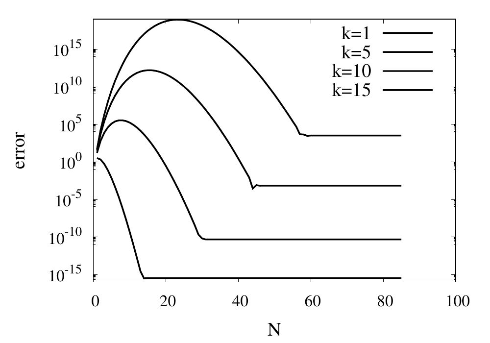
For small values of \(k\), this series converges relatively quickly. But for larger \(k\) you can see that more and more terms are needed. The error even grows first before being reduced. Just like the example above, the truncation error requires large values of \(N\) to reach a good accuracy of the result. In practice, you would not calculate the \(\sin\) function this way. Instead you would make use of known properties, such as \(\sin(2k\pi + x) = \sin(x)\) for integer \(k\), to transform the argument into a range where fast convergence is guaranteed.
However, I would like to continue my analysis of this function because it shows two more interesting pitfalls when performing long sums. First, you will notice that the curves in the figure above show dashed lines for \(N>85\). This is because the implementation I showed above will actually fail with a range error. The pow function and the factorial both start producing numbers that exceed the valid range of double floating-point numbers. The quotient of the two, on the other hand, remains well-behaved. It is, therefore, better to write the Taylor series using a recursive definition of the terms.
\[
\sin x = \sum_{n=0}^\infty a_n(x),
\] with \[
a_0 = x
\] and \[
a_{n} = -\frac{x^2}{2n(2n+1)}a_{n-1}
\]
The implementations are given again below.
C++
double taylor_sin_opt(double x, int order)
{
  double sum = x;
  double an = x;

  for (unsigned int n=1; n<order; ++n)
  {
    an = -x*x*an/(2*n*(2*n+1));
    sum += an;
  }

  return sum;
}
Python
def taylor_sin_opt(x, N):
  sum = x
  an = x

  for n in range(1,N):
    an = -x*x*an/(2*n*(2*n+1))
    sum = sum + an

  return sum
JavaScript
function taylor_sin_opt(x, N) {
  let sum = x;
  let an = x;

  for (let n=1; n<N; n++) {
    an = -x*x*an/(2*n*(2*n+1));
    sum += an;
  }

  return sum;
}
The other takeaway from the graphs of the errors is that they don’t always converge to machine accuracy. The reason for this originates from fact that the initial terms of the sum can be quite large but with opposite signs. They should cancel each other out exactly, but they don’t because of numerical round-off errors.

Computational Physics Basics: Accuracy and Precision
Posted 24th August 2021 by Holger Schmitz
Problems in physics almost always require us to solve mathematical equations with real-valued solutions, and more often than not we want to find functional dependencies of some quantity of a real-valued domain. Numerical solutions to these problems will only ever be approximations to the exact solutions. When a numerical outcome of the calculation is obtained it is important to be able to quantify to what extent it represents the answer that was sought. Two measures of quality are often used to describe numerical solutions: accuracy and precision. Accuracy tells us how will a result agrees with the true value and precision tells us how reproducible the result is. In the standard use of these terms, accuracy and precision are independent of each other.
Accuracy
Accuracy refers to the degree to which the outcome of a calculation or measurement agrees with the true value. The technical definition of accuracy can be a little confusing because it is somewhat different from the everyday use of the word. Consider a measurement that can be carried out many times. A high accuracy implies that, on average, the measured value will be close to the true value. It does not mean that each individual measurement is near the true value. There can be a lot of spread in the measurements. But if we only perform the measurement often enough, we can obtain a reliable outcome.
Precision
Precision refers to the degree to which multiple measurements agree with each other. The term precision in this sense is orthogonal to the notion of accuracy. When carrying out a measurement many times high precision implies that the outcomes will have a small spread. The measurements will be reliable in the sense that they are similar. But they don’t necessarily have to reflect the true value of whatever is being measured.
Accuracy vs Precision
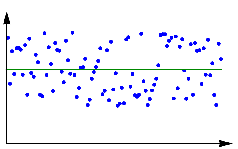
Data with high accuracy but low precision. The green line represents the true value.
To fully grasp the concept of accuracy vs precision it is helpful to look at these two plots. The crosses represent measurements whereas the line represents the true value. In the plot above, the measurements are spread out but they all lie around the true value. These measurements can be said to have low precision but high accuracy. In the plot below, all measurements agree with each other, but they do not represent the true value. In this case, we have high precision but low accuracy.
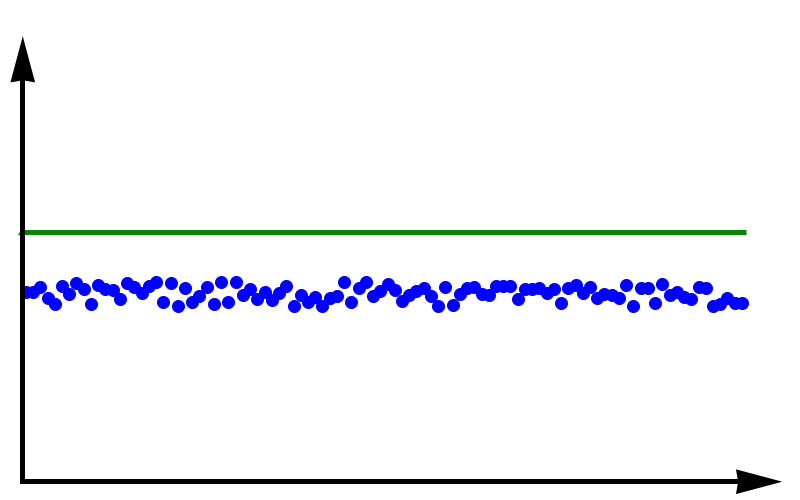
Data with high precision but low accuracy. The green line represents the true value.
A moral can be gained from this: just because you always get the same answer doesn’t mean the answer is correct.
When thinking about numerical methods you might object that calculations are deterministic. Therefore the outcome of repeating a calculation will always be the same. But there is a large class of algorithms that are not quite so deterministic. They might depend on an initial guess or even explicitly on some sequence of pseudo-random numbers. In these cases, repeating the calculation with a different guess or random sequence will lead to a different result.