Computational Physics Basics: Polynomial Interpolation
Posted 19th April 2023 by Holger Schmitz
The piecewise constant interpolation and the linear interpolation seen in the previous post can be understood as special cases of a more general interpolation method. Piecewise constant interpolation constructs a polynomial of order 0 that passes through a single point. Linear interpolation constructs a polynomial of order 1 that passes through 2 points. We can generalise this idea to construct a polynomial of order \(n-1\) that passes through \(n\) points, where \(n\) is 1 or greater. The idea is that a higher-order polynomial will be better at approximating the exact function. We will see later that this idea is only justified in certain cases and that higher-order interpolations can actually increase the error when not applied with care.
Existence
The first question that arises is the following. Given a set of \(n\) points, is there always a polynomial of order \(n-1\) that passes through these points, or are there multiple polynomials with that quality? The first question can be answered simply by constructing a polynomial. The simplest way to do this is to construct the Lagrange Polynomial. Assume we are given a set of points, \[
(x_1, y_1), (x_2, y_2) \ldots (x_n, y_n),
\] where all the \(x\)’s are different, i.e. \(x_i \ne x_j\) if \(i \ne j\). Then we observe that the fraction \[
\frac{x – x_j}{x_i – x_j}
\] is zero when \(x = x_j\) and one when \(x = x_i\). Next, let’s choose an index \(i\) and multiply these fractions together for all \(j\) that are different to \(i\), \[
a_i(x) = \frac{x – x_1}{x_i – x_1}\times \ldots\times\frac{x – x_{i-1}}{x_i – x_{i-1}}
\frac{x – x_{i+1}}{x_i – x_{i+1}}\times \ldots\times\frac{x – x_n}{x_i – x_n}.
\] This product can be written a bit more concisely as \[
a_i(x) = \prod_{\stackrel{j=1}{j\ne i}}^n \frac{x – x_j}{x_i – x_j}.
\] You can see that the \(a_i\) are polynomials of order \(n-1\). Now, if \(x = x_i\) all the factors in the product are 1 which means that \(a_i(x_i) = 1\). On the other hand, if \(x\) is any of the other \(x_j\) then one of the factors will be zero and \(a_i(x_j) = 0\) for any \(j \ne i\). Thus, if we take the product \(a_i(x) y_i\) we have a polynomial that passes through the point \((x_i, y_i)\) but is zero at all the other \(x_j\). The final step is to add up all these separate polynomials to construct the Lagrange Polynomial, \[
p(x) = a_1(x)y_1 + \ldots a_n(x)y_n = \sum_{i=1}^n a_i(x)y_i.
\] By construction, this polynomial of order \(n-1\) passes through all the points \((x_i, y_i)\).
Uniqueness
The next question is if there are other polynomials that pass through all the points, or is the Lagrange Polynomial the only one? The answer is that there is exactly one polynomial of order \(n\) that passes through \(n\) given points. This follows directly from the fundamental theorem of algebra. Imagine we have two order \(n-1\) polynomials, \(p_1\) and \(p_2\), that both pass through our \(n\) points. Then the difference, \[
d(x) = p_1(x) – p_2(x),
\] will also be an order \(n-1\) degree polynomial. But \(d\) also has \(n\) roots because \(d(x_i) = 0\) for all \(i\). But the fundamental theorem of algebra asserts that a polynomial of degree \(n\) can have at most \(n\) real roots unless it is identically zero. In our case \(d\) is of order \(n-1\) and should only have \(n-1\) roots. The fact that it has \(n\) roots means that \(d \equiv 0\). This in turn means that \(p_1 = p_2\) must be the same polynomial.
Approximation Error and Runge’s Phenomenon
One would expect that the higher order interpolations will reduce the error of the approximation and that it would always be best to use the highest possible order. One can find the upper bounds of the error using a similar approach that I used in the previous post on linear interpolation. I will not show the proof here, because it is a bit more tedious and doesn’t give any deeper insights. Given a function \(f(x)\) over an interval \(a\le x \le b\) and sampled at \(n+1\) equidistant points \(x_i = a + hi\), with \(i=0, \ldots , n+1\) and \(h = (b-a)/n\), then the order \(n\) Lagrange polynomial that passes through the points will have an error given by the following formula. \[
\left|R_n(x)\right| \leq \frac{h^{n+1}}{4(n+1)} \left|f^{(n+1)}(x)\right|_{\mathrm{max}}
\] Here \(f^{(n+1)}(x)\) means the \((n+1)\)th derivative of the the function \(f\) and the \(\left|.\right|_{\mathrm{max}}\) means the maximum value over the interval between \(a\) and \(b\). As expected, the error is proportional to \(h^{n+1}\). At first sight, this implies that increasing the number of points, and thus reducing \(h\) while at the same time increasing \(n\) will reduce the error. The problem arises, however, for some functions \(f\) whose \(n\)-th derivatives grow with \(n\). The example put forward by Runge is the function \[
f(x) = \frac{1}{1+25x^2}.
\]

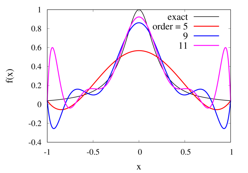
Interpolation of Runge’s function using higher-order polynomials.
The figure above shows the Lagrange polynomials approximating Runge’s function over the interval from -1 to 1 for some orders. You can immediately see that the approximations tend to improve in the central part as the order increases. But near the outermost points, the Lagrange polynomials oscillate more and more wildly as the number of points is increased. The conclusion is that one has to be careful when increasing the interpolation order because spurious oscillations may actually degrade the approximation.
Piecewise Polynomial Interpolation
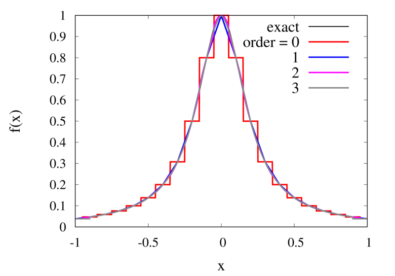
Does this mean we are stuck and that moving to higher orders is generally bad? No, we can make use of higher-order interpolations but we have to be careful. Note, that the polynomial interpolation does get better in the central region when we decrease the spacing between the points. When we used piecewise linear of constant interpolation, we chose the points that were used for the interpolation based on where we wanted to interpolate the function. In the same way, we can choose the points through which we construct the polynomial so that they are always symmetric around \(x\). Some plots of this piecewise polynomial interpolation are shown in the plot below.

Piecewise Lagrange interpolation with 20 points for orders 0, 1, 2, and 3.
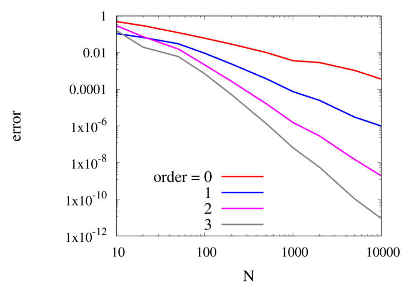
Let’s analyse the error of these approximations. Using an array with \(N\) points on Runge’s function equally spaced between -2 and 2. \(N\) was varied between 10 and 10,000. For each \(N\), the centred polynomial interpolation of orders 0, 1, 2, and 3 was created. Finally, the maximum error of the interpolation and the exact function over the interval -1 and 1 are determined.

Scaling of the maximum error of the Lagrange interpolation with the number of points for increasing order.
The plot above shows the double-logarithmic dependence of the error against the number of points for each order interpolation. The slope of each curve corresponds to the order of the interpolation. For the piecewise constant interpolation, an increase in the number of points by 3 orders of magnitude also corresponds to a reduction of the error by three orders of magnitude. This indicates that the error is first order in this case. For the highest order interpolation and 10,000 points, the error reaches the rounding error of double precision.
Discontinuities and Differentiability
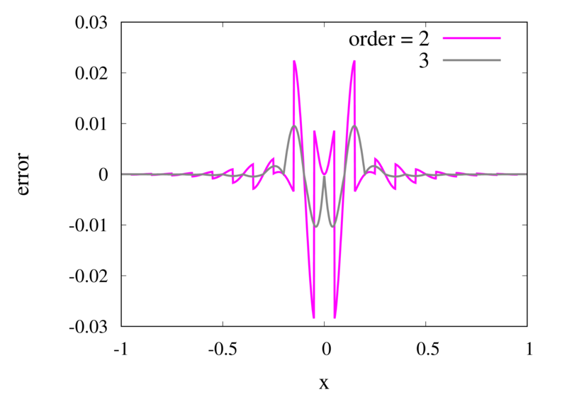
As seen in the previous section, for many cases the piecewise polynomial interpolation can provide a good approximation to the underlying function. However, in some cases, we need to use the first or second derivative of our interpolation. In these cases, the Lagrange formula is not ideal. To see this, the following image shows the interpolation error, again for Runge’s function, using order 2 and 3 polynomials and 20 points.

Error in the Lagrange interpolation of Runge’s function for orders 2 and 3.
One can see that the error in the order 2 approximation has discontinuities and the error in the order 3 approximation has discontinuities of the derivative. For odd-order interpolations, the points that are used for the interpolation change when \(x\) moves from an interval \([x_{i-1},x_i]\) to an interval \([x_i, x_{i+1}]\). Because both interpolations are the same at the point \(x_i\) itself, the interpolation is continuous but the derivative, in general, is not. For even-order interpolations, the stencil changes halfway between the points, which means that the function is discontinuous there. I will address this problem in a future post.