The Euler Equations

Posted 3rd September 2020 by Holger

Leonhard Euler was not only brilliant but also a very productive mathematician. In this post, I want to talk about one of the many things named after the Swiss genius, the Euler equations. These should not be confused with the Euler identity, that famous relation involving $e$, $i$, and $\pi$. No, the Euler equations are a set of partial differential equations that can be used to describe fluid flow. They are related to the Navier-Stokes equations which are at the heart of one of the unsolved Millenium Problems of the Clay Mathematics Institute.

In this short series of posts, I want to present a phenomenological derivation of the equations in one dimension. This derivation is not mathematically rigorous, but will hopefully give you an understanding of the physics that the equations are describing.

Conservation Laws

One way to understand the Euler equations is to write them in the form of conservation laws. Each equation represents a basic conservation law of physics. A central concept in these conservation equation is flux. In a 1d description, the flux of a quantity is a measure for the amount of that quantity that passes through a point. In 2d it’s the amount passing through a line and in 3d through a surface, but let’s stick to 1d during this article.

Take some quantity $N$. To make it concrete, imagine something like the total mass or number of atoms in a volume. I am using the word volume loosely. In 1d a volume is the same as an interval. Let’s call the flux of this quantity $F$. The flux can be different at different locations, so $F$ is a function of position $x$, in other words, the flux is $F(x)$.

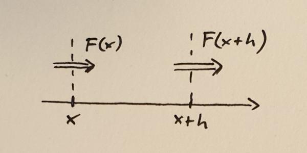
Flux into and out of a small volume between $x$ and $x+h$

Next, consider a small volume between $x$ and $x+h$. Here $h$ is the width of the volume and you should think of it as a small quantity. The rate of change of the quantity $N$ within this volume is determined by the difference between the flux into the volume and the flux out of the volume. If we take positive flux to mean that the quantity (mass, number of atoms, stuff) is moving to the right, then we can write down the following equation.

$$\frac{dN}{dt} = F(x) – F(x+h)$$

Here the left-hand side of the equation represents the rate of change of $N$. I have not written it here but, of course, $N$ depends on the position $x$ as well as the with of the volume $h$. The next step to turn this into a conservation equation is to divide both sides by $h$.

$$\frac{d}{dt}\left(\frac{N}{h}\right) = -\frac{F(x+h) – F(x)}{h}$$

If you remember your calculus lessons, you might already see where this is going. We now make $h$ smaller and smaller and look at the limit when $h \to 0$. The right hand side of the equation will give us the derivative of $F$,
$$\lim_{h \to 0} \frac{F(x+h) – F(x)}{h} = \frac{dF}{dx}$$

The amount of stuff $N$ in the volume will shrink and shrink as $h$ decreases, but because we are dividing by $h$ the ratio $N/h$ will converge to a sensible value. Let’s call this value $n$,

$$n = \lim_{h \to 0}\frac{N}{h}.$$

The quantity $n$ is called the density of $N$. Now the conservation law is simply written as

$$\frac{\partial n}{\partial t} = -\frac{\partial F}{\partial x}.$$

This equation expresses the change of the density of the conserved quantity through the derivative of the flux of that quantity.

The Equations

Now that the basic form of the conservation equations is established, let’s look at some quantities that are conserved and that can be used to express fluid flow. The first conservation law to look at is the conservation of mass. Note again that the conservation equation is written in terms of the density of the conserved quantity. The mass density is the mass contained in a small volume divided by that volume. It is often abbreviated by the Greek letter $\rho$ (rho).

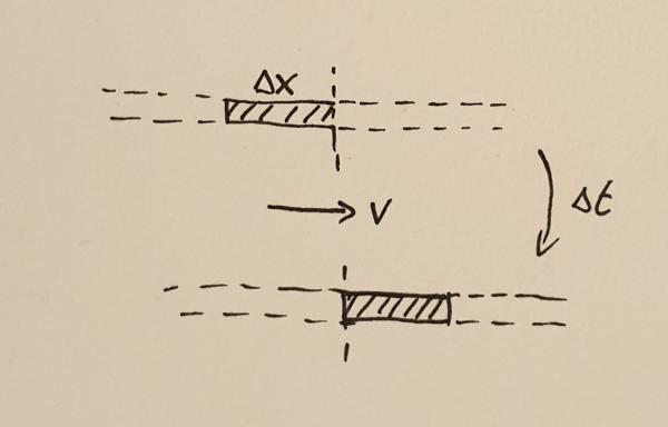
Matter crossing a point during the time interval $\Delta t$

In order to find out what the mass flux is, consider the fluid moving with velocity $v$ through some point. During a small time interval, $\Delta t$ the fluid will move by a small distance $\Delta x$. All the mass $M$ contained in the interval of width $\Delta x$ will cross the point. This mass can be calculated to be

$$M = \rho \Delta x.$$

The flux is the amount of mass crossing the point divided by the time it took the mass to cross that point, $F_{\rho} = M / \Delta t$. In other words,

$$F_{\rho} = \rho \frac{\Delta x}{\Delta t} = \rho v.$$

This now lets us write the mass conservation equation,

$$\frac{\partial \rho}{\partial t} = -\frac{\partial }{\partial x}(\rho v).$$

What does this equation mean? Let me explain this with two examples. First, imagine a constant flow velocity $v$ but an increasing density profile $\rho(x)$. At any given point the density will decrease because the density profile will constantly move towards the right without changing shape. The lower density that was previously located at somewhat left of $x$ will move to the point $x$ thus decreasing the density there.

For the other example, imagine that the density is constant but the velocity has an increasing profile. Matter to the right will flow faster than matter to the left. This will also decrease the density over time because the existing mass is constantly thinned out.

The next conservation equation expresses the conservation of momentum. Momentum is mass times velocity and therefore momentum density is mass density times velocity, $\rho v$. In the mass conservation equation, you could see that the flux consists only of the conserved density multiplied with the velocity. This is called the convective term and this term is present in all Euler equations. However, the momentum can also change through a force. Without external forces, the only force onto each fluid element is through the pressure $p$. The momentum conservation equation can be written as

$$\frac{\partial }{\partial t}(\rho v) = -\frac{\partial }{\partial x}(\rho v^2 + p).$$

The last conservation equation is the conservation of energy, expressed by the energy density $e$,

$$\frac{\partial e}{\partial t} = -\frac{\partial }{\partial x}(e v + p v).$$

The first term is again the convective term expressing the transport of energy contained in the fluid as the fluid moves. The second term is the work done by the pressure force. Note that the energy density $e$ contains the internal (heat) energy as well as the kinetic energy of the fluid moving as a whole.

Finally, we need to close the set of equations by defining what the pressure $p$ is. This closure depends on the type of fluid you want to model. For an ideal gas, the pressure is related to the other variables through

$$p = (\gamma – 1)\left(E – \frac{\rho v^2}{2}\right).$$

Here $\gamma$ is the adiabatic gas index. The second bracket on the right-hand side is the internal energy, expressed as the total energy minus the kinetic energy of the flow.

Putting it All Together

In summary, the Euler equations are conservation equations for the mass, momentum, and energy in the system. In 1d, they can be written as

$$\begin{eqnarray}
\frac{\partial }{\partial t}\rho &=& -\frac{\partial }{\partial x}(\rho v) \\
\frac{\partial }{\partial t}(\rho v) &=& -\frac{\partial }{\partial x}(\rho v^2 + p) \\
\frac{\partial }{\partial t}e &=& -\frac{\partial }{\partial x}(e v + p v)
\end{eqnarray}
$$

In higher dimensions, the derivative with respect to $x$ is replaced by the divergence operator $\nabla$.

$$\begin{eqnarray}
\frac{\partial }{\partial t}\rho &=& -\nabla(\rho \mathbf{v}) \\
\frac{\partial }{\partial t}(\rho v) &=& -\nabla(\rho \mathbf{v}\otimes\mathbf{v} + p\mathbf{I}) \\
\frac{\partial }{\partial t}e &=& -\nabla(e \mathbf{v} + p \mathbf{v})
\end{eqnarray}
$$

The $\otimes$ symbol denotes the outer product of the velocity vectors. It multiplies two vectors to produce a matrix. I will not go into the definition of the outer product here. You can read more on Wikipedia. The symbol $\mathbf{I}$ is the identity matrix.

Summary

The Euler equations are a set of partial differential equations describing fluid flow. When Euler published a simpler version of these equations, they were one of the earliest examples of partial differential equations. Today, the Euler equations and their generalisations, including the Navier-Stokes equations provide the basis for understanding fluid behaviour, turbulence, and the weather.

The Euler equations are difficult to solve and only some special solutions can be written down on paper. For the general case, we need computers to give us answers. In the next post, I will show the results of some simulations I have created with my freely available fluid code Vellamo.