Computational Physics Basics: Piecewise and Linear Interpolation
Posted 24th February 2022 by Holger
One of the main challenges of computational physics is the problem of representing continuous functions in time and space using the finite resources supplied by the computer. A mathematical function of one or more continuous variables naturally has an infinite number of degrees of freedom. These need to be reduced in some manner to be stored in the finite memory available. Maybe the most intuitive way of achieving this goal is by sampling the function at a discrete set of points. We can store the values of the function as a lookup table in memory. It is then straightforward to retrieve the values at the sampling points. However, in many cases, the function values at arbitrary points between the sampling points are needed. It is then necessary to interpolate the function from the given data.
Apart from the interpolation problem, the pointwise discretisation of a function raises another problem. In some cases, the domain over which the function is required is not known in advance. The computer only stores a finite set of points and these points can cover only a finite domain. Extrapolation can be used if the asymptotic behaviour of the function is known. Also, clever spacing of the sample points or transformations of the domain can aid in improving the accuracy of the interpolated and extrapolated function values.
In this post, I will be talking about the interpolation of functions in a single variable. Functions with a higher-dimensional domain will be the subject of a future post.
Functions of a single variable
A function of a single variable, \(f(x)\), can be discretised by specifying the function values at sample locations \(x_i\), where \(i=1 \ldots N\). For now, we don’t require these locations to be evenly spaced but I will assume that they are sorted. This means that \(x_i < x_{i+1}\) for all \(i\). Let’s define the function values, \(y_i\), as \[
y_i = f(x_i).
\] The intuitive idea behind this discretisation is that the function values can be thought of as a number of measurements. The \(y_i\) provide incomplete information about the function. To reconstruct the function over a continuous domain an interpolation scheme needs to be specified.
Piecewise Constant Interpolation
The simplest interpolation scheme is the piecewise constant interpolation, also known as the nearest neighbour interpolation. Given a location \(x\) the goal is to find a value of \(i\) such that \[
|x-x_i| \le |x-x_j| \quad \text{for all} \quad j\ne i.
\] In other words, \(x_i\) is the sample location that is closest to \(x\) when compared to the other sample locations. Then, define the interpolation function \(p_0\) as \[
p_0(x) = f(x_i)
\] with \(x_i\) as defined above. The value of the interpolation is simply the value of the sampled function at the sample point closest to \(x\).
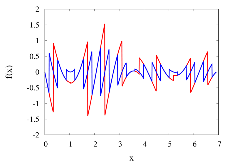
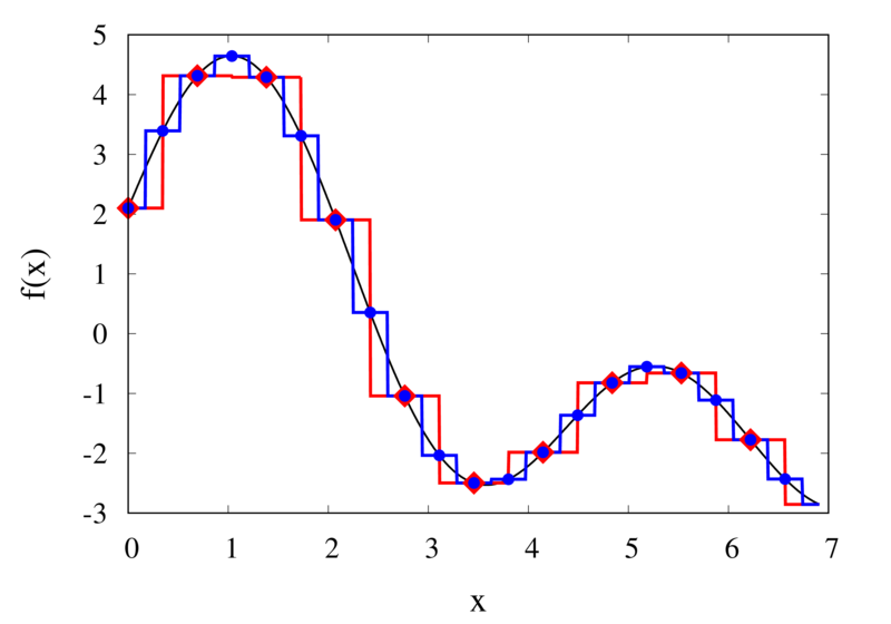
Piecewise constant interpolation of a function (left) and the error (right)
The left plot in the figure above shows some smooth function in black and a number of sample points. The case where 10 sample points are taken is shown by the diamonds and the case for 20 sample points is shown by the circles. Also shown are the nearest neighbour interpolations for these two cases. The red curve shows the interpolated function for 10 samples and the blue curve is for the case of 20 samples. The right plot in the figure shows the difference between the original function and the interpolations. Again, the red curve is for the case of 10 samples and the blue curve is for the case of 20 samples. We can see that the piecewise constant interpolation is crude and the errors are quite large.
As expected, the error is smaller when the number of samples is increased. To analyse exactly how big the error is, consider the residual for the zero-order interpolation \[
R_0(x) = f(x) – p_0(x) = f(x) – f(x_i).
\] The first step to analyse the magnitude of the residual is to perform a Taylor expansion of the residual around the point \(x_i\). We only need the zero order term. Using Taylor’s Theorem and the Cauchy form of the remainder, one can write \[
R_0(x) = \left[ f(x_i) + f'(\xi_c)(x – x_i)\right] – f(x_i).
\] The term in the brackets is the Taylor expansion of \(f(x)\), and \(\xi_c\) is some value that lies between \(x_i\) and \(x\) and depends on the value of \(x\). Let’s define the distance between two samples with \(h=x_{i+1}-x_i\). Assume for the moment that all samples are equidistant. It is not difficult to generalise the arguments for the case when the support points are not equidistant. This means, the maximum value of \(x – x_i\) is half of the distance between two samples, i.e. \[
x – x_i \le \frac{h}{2}.
\] It os also clear that \(f'(\xi_c) \le |f'(x)|_{\mathrm{max}}\), where the maximum is over the interval \(|x-x_i| \le h/2\). The final result for an estimate of the residual error is \[
|R_0(x)| \le\frac{h}{2} |f'(x)|_{\mathrm{max}}
\]
Linear Interpolation
As we saw above, the piecewise interpolation is easy to implement but the errors can be quite large. Most of the time, linear interpolation is a much better alternative. For functions of a single argument, as we are considering here, the computational expense is not much higher than the piecewise interpolation but the resulting accuracy is much better. Given a location \(x\), first find \(i\) such that \[
x_i \le x < x_{i+1}.
\] Then the linear interpolation function \(p_1\) can be defined as \[
p_1(x) = \frac{x_{i+1} – x}{x_{i+1} – x_i} f(x_i)
+ \frac{x – x_i}{x_{i+1} – x_i} f(x_{i+1}).
\] The function \(p_1\) at a point \(x\) can be viewed as a weighted average of the original function values at the neighbouring points \(x_i\) and \(x_{i+1}\). It can be easily seen that \(p(x_i) = f(x_i)\) for all \(i\), i.e. the interpolation goes through the sample points exactly.
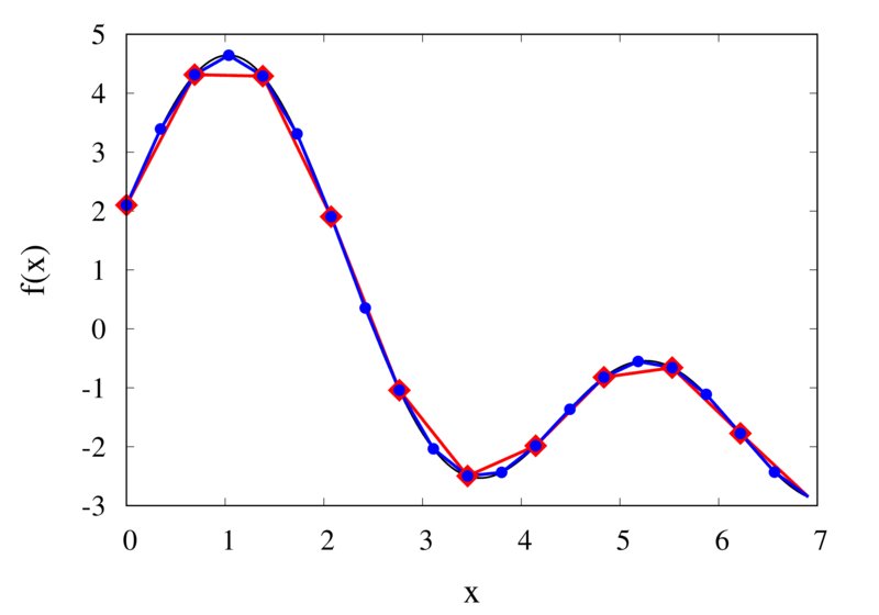
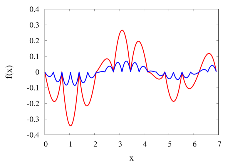
Linear interpolation of a function (left) and the error (right)
The left plot in the figure above shows the same function \(f(x)\) as the figure in the previous section but now together with the linear interpolations for 10 samples (red curve) and 20 samples (blue curve). One can immediately see that the linear interpolation resembles the original function much more closely. The right plot shows the error for the two interpolations. The error is much smaller when compared to the error for the piecewise interpolation. For the 10 sample interpolation, the maximum absolute error of the linear interpolation is about 0.45 compared to a value of over 1.5 for the nearest neighbour interpolation. What’s more, going from 10 to 20 samples improves the error substantially.
One can again try to quantify the error of the linear approximation using Taylor’s Theorem. The first step is to use the Mean Value Theorem that states that there is a point \(x_c\) between \(x_i\) and \(x_{i+1}\) that satisfies \[
f'(x_c) = \frac{ f(x_{i+1}) – f(x_i) }{ x_{i+1} – x_i }.
\] Consider now the error of the linear approximation, \[
R_1(x) = f(x) – p_1(x) = f(x) – \left[\frac{x_{i+1} – x}{x_{i+1} – x_i} f(x_i)
+ \frac{x – x_i}{x_{i+1} – x_i} f(x_{i+1})\right].
\] The derivative of the error is \[
R’_1(x) = f'(x) – \frac{ f(x_{i+1}) – f(x_i) }{ x_{i+1} – x_i }.
\] The Mean Value Theorem implies that the derivative of the error at \(x_c\) is zero and the error is at its maximum at that point. In other words, to estimate the maximum error, we only need to find an upper bound of \(|R(x_c)|\).
We now perform a Taylor expansion of the error around \(x_c\). Using again the Cauchy form of the remainder, we find \[
R(x) = R(x_c) + xR'(x_c) + \frac{1}{2}R’^\prime(\xi_c)(x-\xi_c)(x-x_c).
\] The second term on the right hand side is zero by construction, and we have \[
R(x) = R(x_c) + \frac{1}{2}R’^\prime(\xi_c)(x-\xi_c)(x-x_c).
\] Let \(h\) again denote the distance between the two points, \(h=x_{i+1} – x_i\). We assume that \(x_c – x_i < h/2\) and use the equation above to calculate \(R(x_i)\) which we know is zero. If \(x_c\) was closer to \(x_{i+1}\) we would have to calculate \(R(x_{i+1})\) but otherwise the argument would remain the same. So, \[
R(x_i) = 0 = R(x_c) + \frac{1}{2}R’^\prime(\xi_c)(x_i-\xi_c)(x_i-x_c)
\] from which we get \[
|R(x_c)| = \frac{1}{2}|R’^\prime(\xi_c)(x_i-\xi_c)(x_i-x_c)|.
\] To get an upper estimate of the remainder that does not depend on \(x_c\) or \(\xi_c\) we can use the fact that both \(x_i-\xi_c \le h/2\) and \(x_i-x_c \le h/2\). We also know that \(|R(x)| \le |R(x_c)|\) over the interval from \(x_i\) to \(x_{i+1}\) and \(|R’^\prime(\xi_c)| = |f’^\prime(\xi_c)| \le |f’^\prime(x)|_{\mathrm{max}}\). Given all this, we end up with \[
|R(x)| \le \frac{h^2}{8}|f’^\prime(x)|_{\mathrm{max}}.
\]
The error of the linear interpolation scales with \(h^2\), in contrast to \(h\) for the piecewise constant interpolation. This means that increasing the number of samples gives us much more profit in terms of accuracy. Linear interpolation is often the method of choice because of its relative simplicity combined with reasonable accuracy. In a future post, I will be looking at higher-order interpolations. These higher-order schemes will scale even better with the number of samples but this improvement comes at a cost. We will see that the price to be paid is not only a higher computational expense but also the introduction of spurious oscillations that are not present in the original data.
Leave a Reply