Computational Physics: Truncation and Rounding Errors
Posted 15th October 2021 by Holger
In a previous post, I talked about accuracy and precision in numerical calculations. Ideally one would like to perform calculations that are perfect in these two aspects. However, this is almost never possible in practical situations. The reduction of accuracy or precision is due to two numerical errors. These errors can be classified into two main groups, round-off errors and truncation errors.
Rounding Error
Round-off errors occur due to the limits of numerical precision at which numbers are stored in the computer. As I discussed here a 32-bit floating-point number for example can only store up to 7 or 8 decimal digits. Not just the final result but every intermediate result of a calculation will be rounded to this precision. In some cases, this can result in a much lower precision of the final result. One instance where round-off errors can become a problem happens when the result of a calculation is given by the difference of two large numbers.
Truncation Error
Truncation errors occur because of approximations the numerical scheme makes with respect to the underlying model. The name truncation error stems from the fact that in most schemes the underlying model is first expressed as an infinite series which is then truncated allowing it to be calculated on a computer.
Example: Approximating Pi
Let’s start with a simple task. Use a series to approximate the value of \(\pi\).
Naive summation
One of the traditional ways of calculating \(\pi\) is by using the \(\arctan\) function together with the identity \[
\arctan(1) = \frac{\pi}{4}.
\] One can expand \(\arctan\) into its Taylor series, \[
\arctan(x)
= x – \frac{x^3}{3} +\frac{x^5}{5} – \frac{x^7}{7} + \ldots
= \sum_{n=0}^\infty \frac{(-1)^n x^{2n+1}}{2n+1}.
\] The terms of the series become increasingly smaller and you could try to add up all the terms up to some maximum \(N\) in the hope that the remaining infinite sum is small and can be neglected. Inserting \(x=1\) into the sum will give you an approximation for \(\pi\), \[
\pi \approx 4\sum_{n=0}^N \frac{(-1)^n }{2n+1}.
\]
Here are e implementations for this approximation in C++, Python and JavaScript.
C++
double pi_summation_slow(int N) {
  double  sum = 0.0;
  int  sign = 1;

  for (int  i=0; i<N; ++i) {
    sum += sign/(2*i + 1.0);
    sign = -sign;
  }

  return 4*sum;
}
Python
def  pi_summation_slow(N):
  sum  =  0.0
  sign  =  1

  for  i  in  range(0,N):
    sum   =  sum  +  sign/(2*i  +  1.0)
    sign  =  -sign
    return  4*sum
JavaScript
function pi_summation_slow(N) {
  let sum = 0.0;
  let sign = 1;

  for (let i=0; i<N; ++i) {
    sum += sign/(2*i + 1.0);
    sign = -sign;
  }

  return 4*sum;
}
Let’s call this function with \(N=10\). All the results I am showing here are calculated using a Python implementation. We get a result of around 3.0418. The relative error is 0.0318 and is, of course, unacceptable. This error falls under the category of truncation errors because it is caused by not summing up enough terms of the Taylor series. Calling the function with \(N=1000\) gives us a result of 3.14059 with a relative error of \(3.183\times 10^{-4}\). The error has improved but is still far off from the possible \(10^{-14}\) to \(10^{-15}\) achievable in double-precision arithmetic. The figure below shows how the relative error decreases with the number of iterations.
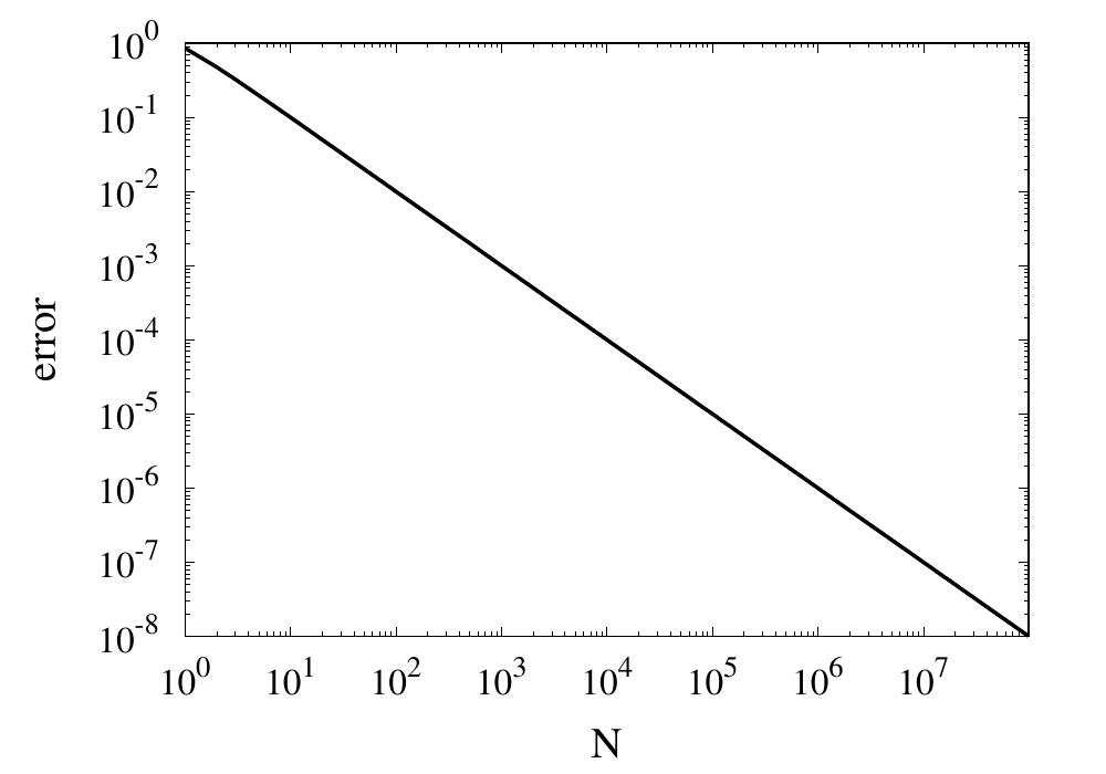
Relative error of the simple approximation of \( \pi \) depending on the number of iterations
From this curve, one h long m wl hat the error decreases with \(1/N\). If one extrapolates the curve, one finds that it would take \(10^{14}\) iterations to reach an error below \(10^{-14}\). Even if this was computationally feasible, the round-off errors of such a long sum would eventually prevent the error from being lowered to this limit.
Improvements using Machin’s formula
The technique of calculating \(\pi\) can be improved in two ways. Firstly, instead of using the Taylor series, you can use Euler’s series for the \(\arctan\) function.
\[
\arctan(x) = \sum_{n=0}^\infty \frac{2^{2n} (n!)^2}{(2n + 1)!} \frac{x^{2n + 1}}{(1 + x^2)^{n + 1}}.
\]
This series converges much more quickly than the Taylor series. The other way to improve convergence is to use trigonometric identities to come up with formulas that converge more quickly. One of the classic equations is the Machin formula for \(\pi\), first discovered by John Machin in 1706, \[
\frac{\pi}{4} = 4 \arctan \frac{1}{5} – \arctan \frac{1}{239}
\] Here are the implementations for this formula.
C++
double pi_summation_fast(int order) {
  using boost::math::factorial;
  double sum = 0.0;

  for (unsigned int n=0; n<order; ++n) {
    double f = factorial<double>(n);
    double common = pow(2.0, 2*n)*f*f/factorial<double>(2*n + 1);
    double A = pow(25./26., n+1)/pow(5., 2*n+1);
    double B = pow(239.*239. / (239.*239. + 1.), n+1)/pow(239., 2*n+1);
    sum += common*( 4*A - B );
  }

  return 4*sum;
}
Python
def pi_summation_fast(N):
  sum = 0.0

  for n in range(0,N):
    f = factorial(n)
    common = math.pow(2.0, 2*n)*f*f/factorial(2*n + 1)
    A = math.pow(25/26, n+1)/math.pow(5, 2*n+1)
    B = math.pow(239*239 / (239*239 + 1), n+1)/math.pow(239, 2*n+1)
    sum = sum + common*( 4*A - B )

  return 4*sum;
JavaScript
function pi_summation_fast(N) {
  let sum = 0.0;

  for (let n=0; n<N; ++n) {
    const f = factorial(n);
    const common = Math.pow(2.0, 2*n)*f*f/factorial(2*n + 1);
    const A = pow(25/26, n+1)/pow(5, 2*n+1);
    const B = pow(239*239 / (239*239 + 1), n+1)/pow(239, 2*n+1);
    sum += common*( 4*A - B );
  }

  return 4*sum;
}
The table below shows the computed values for \(\pi\) together with the relative error. You can see that each iteration reduces the error by more than an order of magnitude and only a few iterations are necessary to achieve machine precision accuracy.
| N | \(S_N\) | error |
|---|---|---|
| 1 | 3.060186968243409 | 0.02591223443732105 |
| 2 | 3.139082236428362 | 0.0007990906009289966 |
| 3 | 3.141509789149037 | 2.6376570705797483e-05 |
| 4 | 3.141589818359699 | 9.024817686074192e-07 |
| 5 | 3.141592554401089 | 3.157274505454055e-08 |
| 6 | 3.141592650066872 | 1.1213806035463463e-09 |
| 7 | 3.1415926534632903 | 4.0267094489200705e-11 |
| 8 | 3.1415926535852132 | 1.4578249079970333e-12 |
| 9 | 3.1415926535896266 | 5.3009244691058615e-14 |
| 10 | 3.1415926535897873 | 1.8376538159566985e-15 |
| 11 | 3.141592653589793 | 0.0 |
Example: Calculating sin(x)
Calculate the value of \(\sin(x)\) using it’s Taylor series around x=0.
The Taylor series for \(\sin(x)\) is \[
\sin x = \sum_{n=0}^\infty \frac{(-1)^n}{(2n+1)!}x^{2n+1}.
\] this series is much more well-behaved than the Taylor series for \(\arctan\) we saw above. Because of the factorial in the denominator, the individual terms of this series will converge reasonably quickly. Here are some naive implementations of this function where the infinite sum has been replaced by a sum from zero to \(N\).
C++
double taylor_sin(double x, int order)
{
  using boost::math::factorial;
  double sum = 0.0;
  int sign = 1;

  for (unsigned int n=0; n<order; ++n)
  {
    sum += sign*pow(x, 2*n + 1)/factorial<double>(2*n +1);
    sign = -sign;
  }

  return sum;
}
Python
def taylor_sin(x, N):
  sum = 0.0
  sign = 1

  for n in range(0,N):
    sum = sum + sign*math.pow(x, 2*n + 1)/factorial(2*n + 1)
    sign = -sign

  return sum
JavaScript
function taylor_sin(x, N) {
  let sum = 0.0;
  let sign = 1;

  for (let n=0; n<N; n++) {
    sum += sign*pow(x, 2*n + 1)/factorial(2*n +1);
    sign = -sign;
  }

  return sum;
}
A good test for this function is the evaluation of \(\sin(x)\) at values \(x = k\pi\), where \(k\) is an integer. We know that \(\sin(k\pi) = 0\) and the return value from the numeric function can directly be used as the absolute error of the computation. The figure below shows results for some values of \(k\) plotted against \(N\).
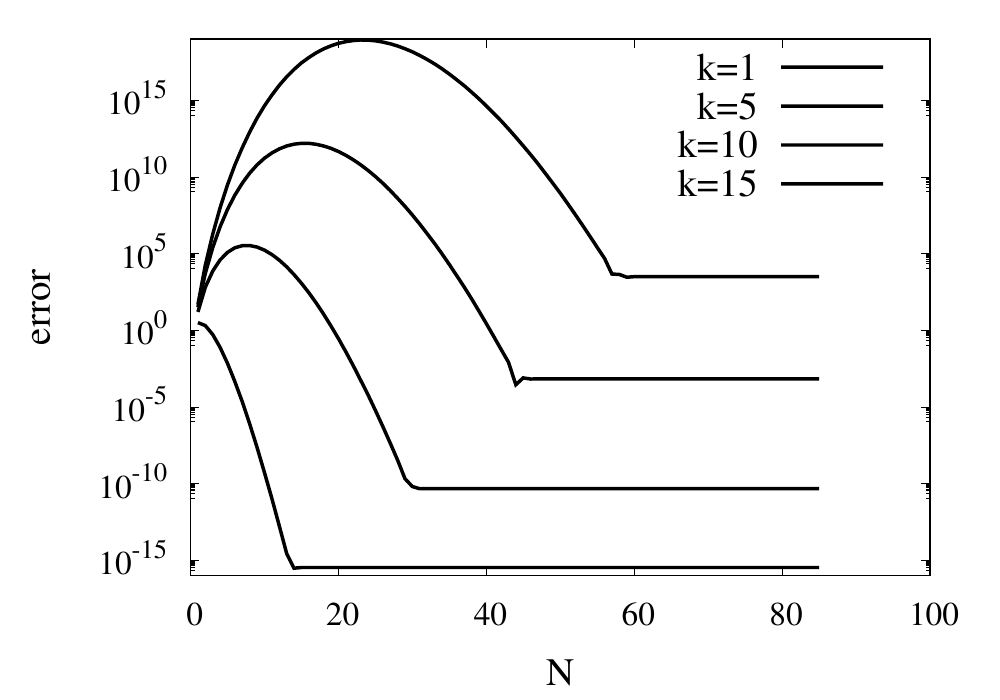
For small values of \(k\), this series converges relatively quickly. But for larger \(k\) you can see that more and more terms are needed. The error even grows first before being reduced. Just like the example above, the truncation error requires large values of \(N\) to reach a good accuracy of the result. In practice, you would not calculate the \(\sin\) function this way. Instead you would make use of known properties, such as \(\sin(2k\pi + x) = \sin(x)\) for integer \(k\), to transform the argument into a range where fast convergence is guaranteed.
However, I would like to continue my analysis of this function because it shows two more interesting pitfalls when performing long sums. First, you will notice that the curves in the figure above show dashed lines for \(N>85\). This is because the implementation I showed above will actually fail with a range error. The pow function and the factorial both start producing numbers that exceed the valid range of double floating-point numbers. The quotient of the two, on the other hand, remains well-behaved. It is, therefore, better to write the Taylor series using a recursive definition of the terms.
\[
\sin x = \sum_{n=0}^\infty a_n(x),
\] with \[
a_0 = x
\] and \[
a_{n} = -\frac{x^2}{2n(2n+1)}a_{n-1}
\]
The implementations are given again below.
C++
double taylor_sin_opt(double x, int order)
{
  double sum = x;
  double an = x;

  for (unsigned int n=1; n<order; ++n)
  {
    an = -x*x*an/(2*n*(2*n+1));
    sum += an;
  }

  return sum;
}
Python
def taylor_sin_opt(x, N):
  sum = x
  an = x

  for n in range(1,N):
    an = -x*x*an/(2*n*(2*n+1))
    sum = sum + an

  return sum
JavaScript
function taylor_sin_opt(x, N) {
  let sum = x;
  let an = x;

  for (let n=1; n<N; n++) {
    an = -x*x*an/(2*n*(2*n+1));
    sum += an;
  }

  return sum;
}
The other takeaway from the graphs of the errors is that they don’t always converge to machine accuracy. The reason for this originates from fact that the initial terms of the sum can be quite large but with opposite signs. They should cancel each other out exactly, but they don’t because of numerical round-off errors.
Leave a Reply