Computational Physics Basics: Polynomial Interpolation
Posted 19th April 2023 by Holger Schmitz
The piecewise constant interpolation and the linear interpolation seen in the previous post can be understood as special cases of a more general interpolation method. Piecewise constant interpolation constructs a polynomial of order 0 that passes through a single point. Linear interpolation constructs a polynomial of order 1 that passes through 2 points. We can generalise this idea to construct a polynomial of order \(n-1\) that passes through \(n\) points, where \(n\) is 1 or greater. The idea is that a higher-order polynomial will be better at approximating the exact function. We will see later that this idea is only justified in certain cases and that higher-order interpolations can actually increase the error when not applied with care.
Existence
The first question that arises is the following. Given a set of \(n\) points, is there always a polynomial of order \(n-1\) that passes through these points, or are there multiple polynomials with that quality? The first question can be answered simply by constructing a polynomial. The simplest way to do this is to construct the Lagrange Polynomial. Assume we are given a set of points, \[
(x_1, y_1), (x_2, y_2) \ldots (x_n, y_n),
\] where all the \(x\)’s are different, i.e. \(x_i \ne x_j\) if \(i \ne j\). Then we observe that the fraction \[
\frac{x – x_j}{x_i – x_j}
\] is zero when \(x = x_j\) and one when \(x = x_i\). Next, let’s choose an index \(i\) and multiply these fractions together for all \(j\) that are different to \(i\), \[
a_i(x) = \frac{x – x_1}{x_i – x_1}\times \ldots\times\frac{x – x_{i-1}}{x_i – x_{i-1}}
\frac{x – x_{i+1}}{x_i – x_{i+1}}\times \ldots\times\frac{x – x_n}{x_i – x_n}.
\] This product can be written a bit more concisely as \[
a_i(x) = \prod_{\stackrel{j=1}{j\ne i}}^n \frac{x – x_j}{x_i – x_j}.
\] You can see that the \(a_i\) are polynomials of order \(n-1\). Now, if \(x = x_i\) all the factors in the product are 1 which means that \(a_i(x_i) = 1\). On the other hand, if \(x\) is any of the other \(x_j\) then one of the factors will be zero and \(a_i(x_j) = 0\) for any \(j \ne i\). Thus, if we take the product \(a_i(x) y_i\) we have a polynomial that passes through the point \((x_i, y_i)\) but is zero at all the other \(x_j\). The final step is to add up all these separate polynomials to construct the Lagrange Polynomial, \[
p(x) = a_1(x)y_1 + \ldots a_n(x)y_n = \sum_{i=1}^n a_i(x)y_i.
\] By construction, this polynomial of order \(n-1\) passes through all the points \((x_i, y_i)\).
Uniqueness
The next question is if there are other polynomials that pass through all the points, or is the Lagrange Polynomial the only one? The answer is that there is exactly one polynomial of order \(n\) that passes through \(n\) given points. This follows directly from the fundamental theorem of algebra. Imagine we have two order \(n-1\) polynomials, \(p_1\) and \(p_2\), that both pass through our \(n\) points. Then the difference, \[
d(x) = p_1(x) – p_2(x),
\] will also be an order \(n-1\) degree polynomial. But \(d\) also has \(n\) roots because \(d(x_i) = 0\) for all \(i\). But the fundamental theorem of algebra asserts that a polynomial of degree \(n\) can have at most \(n\) real roots unless it is identically zero. In our case \(d\) is of order \(n-1\) and should only have \(n-1\) roots. The fact that it has \(n\) roots means that \(d \equiv 0\). This in turn means that \(p_1 = p_2\) must be the same polynomial.
Approximation Error and Runge’s Phenomenon
One would expect that the higher order interpolations will reduce the error of the approximation and that it would always be best to use the highest possible order. One can find the upper bounds of the error using a similar approach that I used in the previous post on linear interpolation. I will not show the proof here, because it is a bit more tedious and doesn’t give any deeper insights. Given a function \(f(x)\) over an interval \(a\le x \le b\) and sampled at \(n+1\) equidistant points \(x_i = a + hi\), with \(i=0, \ldots , n+1\) and \(h = (b-a)/n\), then the order \(n\) Lagrange polynomial that passes through the points will have an error given by the following formula. \[
\left|R_n(x)\right| \leq \frac{h^{n+1}}{4(n+1)} \left|f^{(n+1)}(x)\right|_{\mathrm{max}}
\] Here \(f^{(n+1)}(x)\) means the \((n+1)\)th derivative of the the function \(f\) and the \(\left|.\right|_{\mathrm{max}}\) means the maximum value over the interval between \(a\) and \(b\). As expected, the error is proportional to \(h^{n+1}\). At first sight, this implies that increasing the number of points, and thus reducing \(h\) while at the same time increasing \(n\) will reduce the error. The problem arises, however, for some functions \(f\) whose \(n\)-th derivatives grow with \(n\). The example put forward by Runge is the function \[
f(x) = \frac{1}{1+25x^2}.
\]
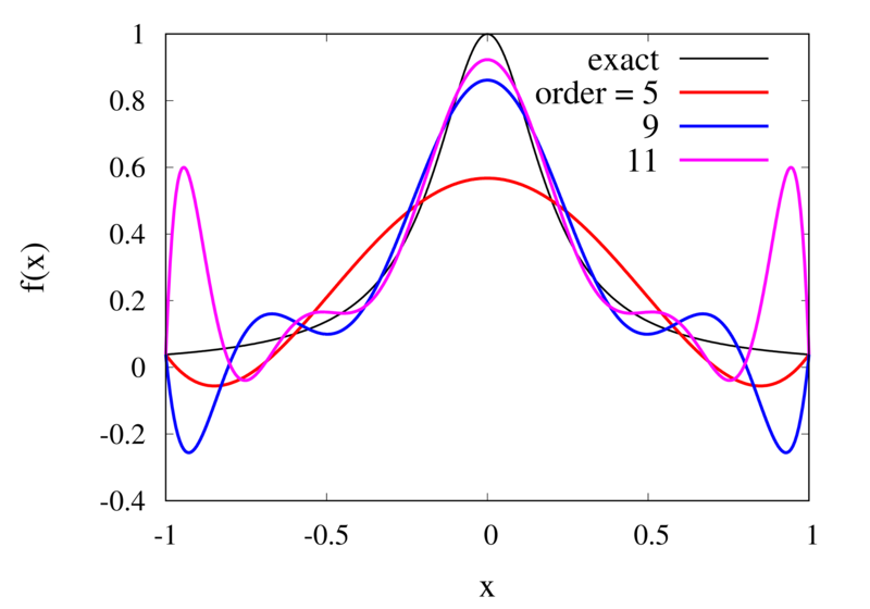
Interpolation of Runge’s function using higher-order polynomials.
The figure above shows the Lagrange polynomials approximating Runge’s function over the interval from -1 to 1 for some orders. You can immediately see that the approximations tend to improve in the central part as the order increases. But near the outermost points, the Lagrange polynomials oscillate more and more wildly as the number of points is increased. The conclusion is that one has to be careful when increasing the interpolation order because spurious oscillations may actually degrade the approximation.
Piecewise Polynomial Interpolation
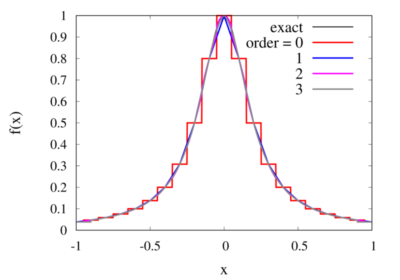
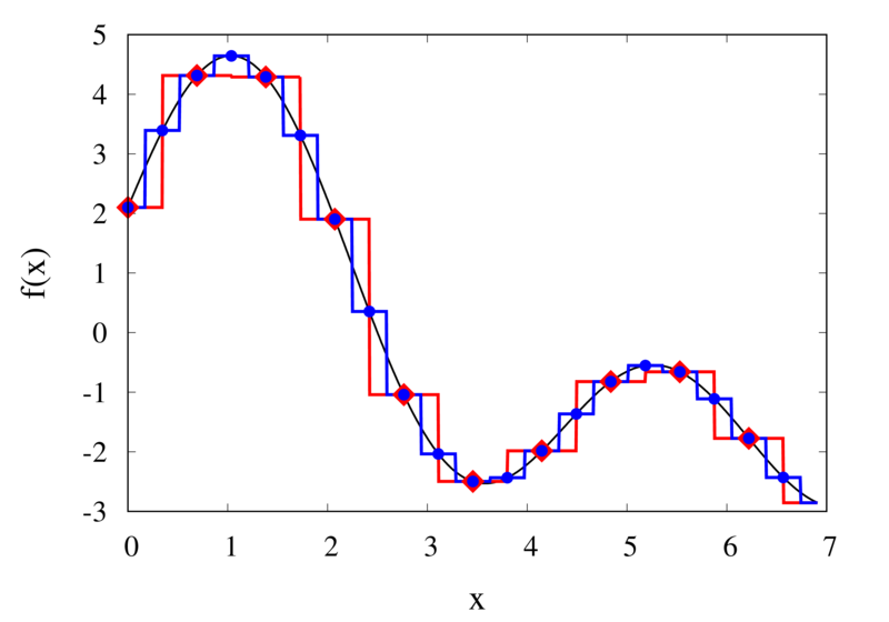
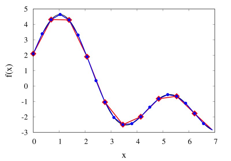
Does this mean we are stuck and that moving to higher orders is generally bad? No, we can make use of higher-order interpolations but we have to be careful. Note, that the polynomial interpolation does get better in the central region when we decrease the spacing between the points. When we used piecewise linear of constant interpolation, we chose the points that were used for the interpolation based on where we wanted to interpolate the function. In the same way, we can choose the points through which we construct the polynomial so that they are always symmetric around \(x\). Some plots of this piecewise polynomial interpolation are shown in the plot below.
Piecewise Lagrange interpolation with 20 points for orders 0, 1, 2, and 3.
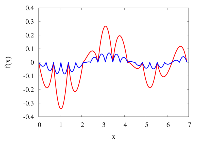
Let’s analyse the error of these approximations. Using an array with \(N\) points on Runge’s function equally spaced between -2 and 2. \(N\) was varied between 10 and 10,000. For each \(N\), the centred polynomial interpolation of orders 0, 1, 2, and 3 was created. Finally, the maximum error of the interpolation and the exact function over the interval -1 and 1 are determined.
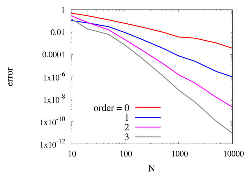
Scaling of the maximum error of the Lagrange interpolation with the number of points for increasing order.
The plot above shows the double-logarithmic dependence of the error against the number of points for each order interpolation. The slope of each curve corresponds to the order of the interpolation. For the piecewise constant interpolation, an increase in the number of points by 3 orders of magnitude also corresponds to a reduction of the error by three orders of magnitude. This indicates that the error is first order in this case. For the highest order interpolation and 10,000 points, the error reaches the rounding error of double precision.
Discontinuities and Differentiability
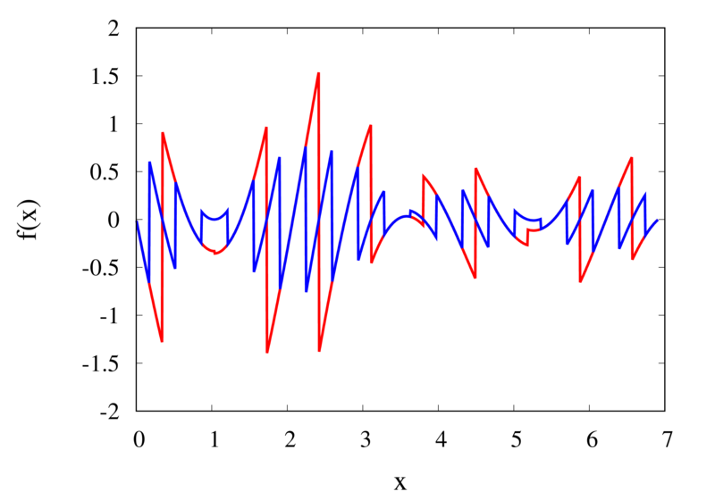
As seen in the previous section, for many cases the piecewise polynomial interpolation can provide a good approximation to the underlying function. However, in some cases, we need to use the first or second derivative of our interpolation. In these cases, the Lagrange formula is not ideal. To see this, the following image shows the interpolation error, again for Runge’s function, using order 2 and 3 polynomials and 20 points.
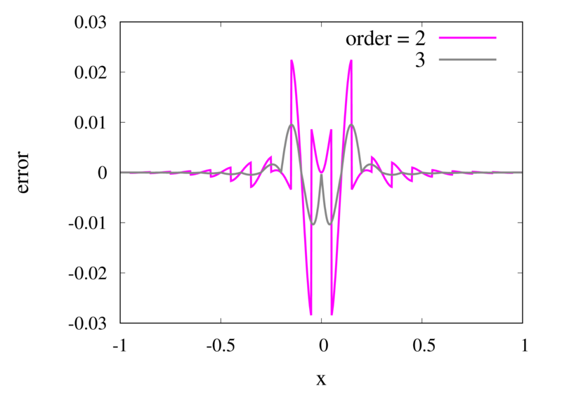
Error in the Lagrange interpolation of Runge’s function for orders 2 and 3.
One can see that the error in the order 2 approximation has discontinuities and the error in the order 3 approximation has discontinuities of the derivative. For odd-order interpolations, the points that are used for the interpolation change when \(x\) moves from an interval \([x_{i-1},x_i]\) to an interval \([x_i, x_{i+1}]\). Because both interpolations are the same at the point \(x_i\) itself, the interpolation is continuous but the derivative, in general, is not. For even-order interpolations, the stencil changes halfway between the points, which means that the function is discontinuous there. I will address this problem in a future post.
Computational Physics Basics: Piecewise and Linear Interpolation
Posted 24th February 2022 by Holger Schmitz
One of the main challenges of computational physics is the problem of representing continuous functions in time and space using the finite resources supplied by the computer. A mathematical function of one or more continuous variables naturally has an infinite number of degrees of freedom. These need to be reduced in some manner to be stored in the finite memory available. Maybe the most intuitive way of achieving this goal is by sampling the function at a discrete set of points. We can store the values of the function as a lookup table in memory. It is then straightforward to retrieve the values at the sampling points. However, in many cases, the function values at arbitrary points between the sampling points are needed. It is then necessary to interpolate the function from the given data.
Apart from the interpolation problem, the pointwise discretisation of a function raises another problem. In some cases, the domain over which the function is required is not known in advance. The computer only stores a finite set of points and these points can cover only a finite domain. Extrapolation can be used if the asymptotic behaviour of the function is known. Also, clever spacing of the sample points or transformations of the domain can aid in improving the accuracy of the interpolated and extrapolated function values.
In this post, I will be talking about the interpolation of functions in a single variable. Functions with a higher-dimensional domain will be the subject of a future post.
Functions of a single variable
A function of a single variable, \(f(x)\), can be discretised by specifying the function values at sample locations \(x_i\), where \(i=1 \ldots N\). For now, we don’t require these locations to be evenly spaced but I will assume that they are sorted. This means that \(x_i < x_{i+1}\) for all \(i\). Let’s define the function values, \(y_i\), as \[
y_i = f(x_i).
\] The intuitive idea behind this discretisation is that the function values can be thought of as a number of measurements. The \(y_i\) provide incomplete information about the function. To reconstruct the function over a continuous domain an interpolation scheme needs to be specified.
Piecewise Constant Interpolation
The simplest interpolation scheme is the piecewise constant interpolation, also known as the nearest neighbour interpolation. Given a location \(x\) the goal is to find a value of \(i\) such that \[
|x-x_i| \le |x-x_j| \quad \text{for all} \quad j\ne i.
\] In other words, \(x_i\) is the sample location that is closest to \(x\) when compared to the other sample locations. Then, define the interpolation function \(p_0\) as \[
p_0(x) = f(x_i)
\] with \(x_i\) as defined above. The value of the interpolation is simply the value of the sampled function at the sample point closest to \(x\).
Piecewise constant interpolation of a function (left) and the error (right)
The left plot in the figure above shows some smooth function in black and a number of sample points. The case where 10 sample points are taken is shown by the diamonds and the case for 20 sample points is shown by the circles. Also shown are the nearest neighbour interpolations for these two cases. The red curve shows the interpolated function for 10 samples and the blue curve is for the case of 20 samples. The right plot in the figure shows the difference between the original function and the interpolations. Again, the red curve is for the case of 10 samples and the blue curve is for the case of 20 samples. We can see that the piecewise constant interpolation is crude and the errors are quite large.
As expected, the error is smaller when the number of samples is increased. To analyse exactly how big the error is, consider the residual for the zero-order interpolation \[
R_0(x) = f(x) – p_0(x) = f(x) – f(x_i).
\] The first step to analyse the magnitude of the residual is to perform a Taylor expansion of the residual around the point \(x_i\). We only need the zero order term. Using Taylor’s Theorem and the Cauchy form of the remainder, one can write \[
R_0(x) = \left[ f(x_i) + f'(\xi_c)(x – x_i)\right] – f(x_i).
\] The term in the brackets is the Taylor expansion of \(f(x)\), and \(\xi_c\) is some value that lies between \(x_i\) and \(x\) and depends on the value of \(x\). Let’s define the distance between two samples with \(h=x_{i+1}-x_i\). Assume for the moment that all samples are equidistant. It is not difficult to generalise the arguments for the case when the support points are not equidistant. This means, the maximum value of \(x – x_i\) is half of the distance between two samples, i.e. \[
x – x_i \le \frac{h}{2}.
\] It os also clear that \(f'(\xi_c) \le |f'(x)|_{\mathrm{max}}\), where the maximum is over the interval \(|x-x_i| \le h/2\). The final result for an estimate of the residual error is \[
|R_0(x)| \le\frac{h}{2} |f'(x)|_{\mathrm{max}}
\]
Linear Interpolation
As we saw above, the piecewise interpolation is easy to implement but the errors can be quite large. Most of the time, linear interpolation is a much better alternative. For functions of a single argument, as we are considering here, the computational expense is not much higher than the piecewise interpolation but the resulting accuracy is much better. Given a location \(x\), first find \(i\) such that \[
x_i \le x < x_{i+1}.
\] Then the linear interpolation function \(p_1\) can be defined as \[
p_1(x) = \frac{x_{i+1} – x}{x_{i+1} – x_i} f(x_i)
+ \frac{x – x_i}{x_{i+1} – x_i} f(x_{i+1}).
\] The function \(p_1\) at a point \(x\) can be viewed as a weighted average of the original function values at the neighbouring points \(x_i\) and \(x_{i+1}\). It can be easily seen that \(p(x_i) = f(x_i)\) for all \(i\), i.e. the interpolation goes through the sample points exactly.
Linear interpolation of a function (left) and the error (right)
The left plot in the figure above shows the same function \(f(x)\) as the figure in the previous section but now together with the linear interpolations for 10 samples (red curve) and 20 samples (blue curve). One can immediately see that the linear interpolation resembles the original function much more closely. The right plot shows the error for the two interpolations. The error is much smaller when compared to the error for the piecewise interpolation. For the 10 sample interpolation, the maximum absolute error of the linear interpolation is about 0.45 compared to a value of over 1.5 for the nearest neighbour interpolation. What’s more, going from 10 to 20 samples improves the error substantially.
One can again try to quantify the error of the linear approximation using Taylor’s Theorem. The first step is to use the Mean Value Theorem that states that there is a point \(x_c\) between \(x_i\) and \(x_{i+1}\) that satisfies \[
f'(x_c) = \frac{ f(x_{i+1}) – f(x_i) }{ x_{i+1} – x_i }.
\] Consider now the error of the linear approximation, \[
R_1(x) = f(x) – p_1(x) = f(x) – \left[\frac{x_{i+1} – x}{x_{i+1} – x_i} f(x_i)
+ \frac{x – x_i}{x_{i+1} – x_i} f(x_{i+1})\right].
\] The derivative of the error is \[
R’_1(x) = f'(x) – \frac{ f(x_{i+1}) – f(x_i) }{ x_{i+1} – x_i }.
\] The Mean Value Theorem implies that the derivative of the error at \(x_c\) is zero and the error is at its maximum at that point. In other words, to estimate the maximum error, we only need to find an upper bound of \(|R(x_c)|\).
We now perform a Taylor expansion of the error around \(x_c\). Using again the Cauchy form of the remainder, we find \[
R(x) = R(x_c) + xR'(x_c) + \frac{1}{2}R’^\prime(\xi_c)(x-\xi_c)(x-x_c).
\] The second term on the right hand side is zero by construction, and we have \[
R(x) = R(x_c) + \frac{1}{2}R’^\prime(\xi_c)(x-\xi_c)(x-x_c).
\] Let \(h\) again denote the distance between the two points, \(h=x_{i+1} – x_i\). We assume that \(x_c – x_i < h/2\) and use the equation above to calculate \(R(x_i)\) which we know is zero. If \(x_c\) was closer to \(x_{i+1}\) we would have to calculate \(R(x_{i+1})\) but otherwise the argument would remain the same. So, \[
R(x_i) = 0 = R(x_c) + \frac{1}{2}R’^\prime(\xi_c)(x_i-\xi_c)(x_i-x_c)
\] from which we get \[
|R(x_c)| = \frac{1}{2}|R’^\prime(\xi_c)(x_i-\xi_c)(x_i-x_c)|.
\] To get an upper estimate of the remainder that does not depend on \(x_c\) or \(\xi_c\) we can use the fact that both \(x_i-\xi_c \le h/2\) and \(x_i-x_c \le h/2\). We also know that \(|R(x)| \le |R(x_c)|\) over the interval from \(x_i\) to \(x_{i+1}\) and \(|R’^\prime(\xi_c)| = |f’^\prime(\xi_c)| \le |f’^\prime(x)|_{\mathrm{max}}\). Given all this, we end up with \[
|R(x)| \le \frac{h^2}{8}|f’^\prime(x)|_{\mathrm{max}}.
\]
The error of the linear interpolation scales with \(h^2\), in contrast to \(h\) for the piecewise constant interpolation. This means that increasing the number of samples gives us much more profit in terms of accuracy. Linear interpolation is often the method of choice because of its relative simplicity combined with reasonable accuracy. In a future post, I will be looking at higher-order interpolations. These higher-order schemes will scale even better with the number of samples but this improvement comes at a cost. We will see that the price to be paid is not only a higher computational expense but also the introduction of spurious oscillations that are not present in the original data.
Frege’s Numbers
Posted 19th November 2021 by Holger Schmitz
In a previous post, I started talking about natural numbers and how the Peano axioms define the relation between natural numbers. These axioms allow you to work with numbers and are good enough for most everyday uses. From a philosophical point of view, the Peano axioms have one big drawback. They only tell us how natural numbers behave but they don’t say anything about what natural numbers actually are. In the late 19th Century mathematicians started using set theory as the basis to define the axioms of arithmetic and other branches of mathematics. Two mathematicians, first Frege and later Bertrand Russell came up with a definition of natural numbers that gives us some insight into the nature of these elusive objects. In order to understand their definitions, I will first have to make the little excursion into set theory.
You may have encountered the basics of set theory already in primary school. Naïvely speaking sets are collections of things. Often the object in a set share some common property but this is not strictly necessary. You may have drawn Venn diagrams to depict sets, their unions and intersections. Something that is not taught in primary school is that you can define relations between sets that, in turn, define the so-called cardinality of a set.
Functions and Bijections
One of the central concepts is the mapping between two sets. For the following let’s assume we have two sets, \(\mathcal{A}\) and \(\mathcal{B}\). A function simply defines a rule that assigns an element of set \(\mathcal{B}\) to each element of set \(\mathcal{A}\). We call \(\mathcal{A}\) the domain of the function and \(\mathcal{B}\) the range of the function. If the function is named \(f\), then we write \[
f: \mathcal{A} \to \mathcal{B}
\] to indicate what the domain and the range of the function are.
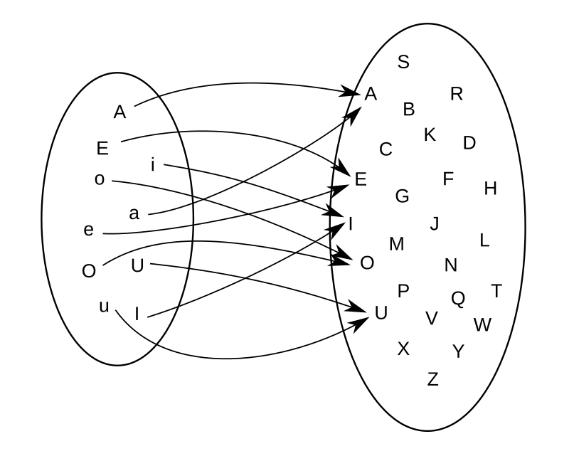
A function that maps vowels to uppercase letters
Example: For example, if \(\mathcal{A}\) is the set of uppercase and lowercase vowels, \[
\mathcal{A} = { A, E, I, O, U, a, e, i, o, u },
\] and \(\mathcal{B}\) is the set of all uppercase letters in the alphabet, \[
\mathcal{B} = { A, B, C, D, \ldots, Z}.
\]
Now we can define a function that assigns the uppercase letter in \(\mathcal{B}\) to each vowel in \(\mathcal{A}\). So the mapping looks like shown in the figure.
You will notice two properties about this function. Firstly, not all elements from \(\mathcal{B}\) appear as a mapping of an element from \(\mathcal{A}\). We say that the uppercase consonants in \(\mathcal{B}\) are not in the image of \(\mathcal{A}\).
The second thing to note is that some elements in \(\mathcal{B}\) appear twice. For example, both the lowercase e and the uppercase E in \(\mathcal{A}\) map to the same uppercase E in \(\mathcal{B}\).
Definition of a Bijection
The example shows a function that is not a bijection. In order to be a bijection, a function must ensure that each element in the range is mapped to by exactly one element from the range. In other words for a function \[
f: \mathcal{A} \to \mathcal{B}
\]
- every element in \(\mathcal{B}\) appears as a function value. No element is left out.
- no element in \(\mathcal{B}\) appears as a function value more than once.
A bijection implies a one-to-one relationship between the elements in set \(\mathcal{A}\) and set \(\mathcal{B}\).
Equinumerosity and Cardinality
Intuitively, it is clear that you can only have a bijection between two sets if they have the same number of elements. After all, each element in \(\mathcal{A}\) is mapped onto exactly one element in \(\mathcal{B}\). This can be used to define a relation between any two sets.
Two sets are called equinumerous if there exists a bijection between the two sets. Equinumerous literally means “having the same number”. But we have to be careful here because we don’t yet know what the term “number” is supposed to mean. That is the reason why we define the term by using bijections and not referring to any “amount” or “number of elements”. Instead of saying that two sets are equinumerous, we can also say that they have the same cardinality.
Now comes the clever bit that Frege proposed. Let’s create a class of sets that all share the same cardinality. We can do that because equinumerosity is an equivalence relation but I won’t go into detail about what that means. We will call this cardinality class \(N\), so \[
N(\mathcal{A})
\] is the class of all the sets that are equinumerous to \(\mathcal{A}\).
Intuitively we now have a class with all the sets that contain exactly one element, another class with all the sets that contain exactly two elements, and so forth. But we don’t know anything about numbers yet, so we also don’t really know what one and two are supposed to mean.
Constructing Natural Numbers
Now we have all the tools to construct the natural numbers \(\mathbb{N}\). Of course, we want our numbers to obey the Peano axioms, so we need two things. We need a zero element and we need a successor function \(S(n)\) that produces the next number from any given number.
The Zero Element
The zero-element is easily defined. We can construct the empty set, \[
\emptyset = \{\}.
\] This is the set with no elements in it. Now the zero-element is simply the cardinality class of the empty set, \[
0 = N(\emptyset).
\] This means that zero is a class of sets that all share the same cardinality as the empty set. You can show that this class consists of only one element, the empty set, by I won’t go into that here.
The Successor Function
Given that we have defined the zero element, \(0\), we can now define a set that contains zero as a single element, \[
\{0\}.
\] Intuitively, this set has one element and we can thus define the natural number \(1\) as the cardinality class of this set, \[
1 = N(\{0\}).
\] In general, given any natural number \(n\) we can define the successor \(S(n)\) by creating the cardinality class of the set that contains \(n\) together with all its predecessors, \[
n+1 = S(n) = N(\{0, 1, \ldots, n\}).
\] You might think that this definition is somewhat circular. We are defining the successor function by using the concept of the predecessors. But this is not as problematic as it might seem at first sight. We know that the predecessor of \(1\) is \(0\) and each time we construct the next natural number, we can keep track of all the predecessors that we have constructed so far.
Conclusion
The zero and the successor function defined above are enough to define all the natural numbers \(\mathbb{N}\). I will not go into the proof that all the Peano axioms are satisfied by this construction. It is relatively straightforward and not very instructive in my opinion. If you want, you can try doing the proof as an exercise.
I personally find the Frege definition of natural numbers the most satisfying. It tells us that a number is not just some random symbol that doesn’t relate to the real world. A natural number is the class of all sets that share the same property. Each set in the class has the same cardinality and we can identify the cardinality with that number. It means that any set of objects in the real world can be thought of as an instance of a number. The number itself is the collection of sets and the concrete set is contained within it as an element. For example, if you see five apples on a table, you can think of them as a manifestation of the number \(5\).

This set of pins is an instance of the number 4 (four).
Another consequence of the definition of cardinality is that it gives us the ability to speak about infinities. A set might have an infinite number of elements. We already encountered \(\mathbb{N}\), the set of all natural numbers. Using the cardinality, we can compare infinite sets and create a hierarchy of infinities. I might talk about this more in a later post.
It would not be fair, however, if I didn’t mention some serious problems with the definition that I Frege came up with. The main problem arises because we are creating classes of sets without explicitly saying which elements we are allowing to be in those sets. This allows sets to contain arbitrary elements, including other sets. A set can even include itself as an element. This leads to the famous paradox by Russel which can be summarised as follows. Construct a set \(\mathcal{R}\) of all the sets that do not include themselves as an element. Then ask the question, does \(\mathcal{R}\) include itself? There are mathematical frameworks that attempt to save the essence of Frege’s definition of the natural numbers without running into these problems. In my personal opinion, they always lose some of the beauty and simplicity. But this is a necessary concession to make if you want to end up with a mathematical framework that doesn’t contain internal contradictions.

Computational Physics Basics: Accuracy and Precision
Posted 24th August 2021 by Holger Schmitz
Problems in physics almost always require us to solve mathematical equations with real-valued solutions, and more often than not we want to find functional dependencies of some quantity of a real-valued domain. Numerical solutions to these problems will only ever be approximations to the exact solutions. When a numerical outcome of the calculation is obtained it is important to be able to quantify to what extent it represents the answer that was sought. Two measures of quality are often used to describe numerical solutions: accuracy and precision. Accuracy tells us how will a result agrees with the true value and precision tells us how reproducible the result is. In the standard use of these terms, accuracy and precision are independent of each other.
Accuracy
Accuracy refers to the degree to which the outcome of a calculation or measurement agrees with the true value. The technical definition of accuracy can be a little confusing because it is somewhat different from the everyday use of the word. Consider a measurement that can be carried out many times. A high accuracy implies that, on average, the measured value will be close to the true value. It does not mean that each individual measurement is near the true value. There can be a lot of spread in the measurements. But if we only perform the measurement often enough, we can obtain a reliable outcome.
Precision
Precision refers to the degree to which multiple measurements agree with each other. The term precision in this sense is orthogonal to the notion of accuracy. When carrying out a measurement many times high precision implies that the outcomes will have a small spread. The measurements will be reliable in the sense that they are similar. But they don’t necessarily have to reflect the true value of whatever is being measured.
Accuracy vs Precision
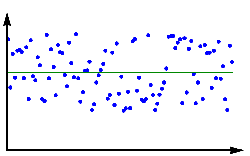
Data with high accuracy but low precision. The green line represents the true value.
To fully grasp the concept of accuracy vs precision it is helpful to look at these two plots. The crosses represent measurements whereas the line represents the true value. In the plot above, the measurements are spread out but they all lie around the true value. These measurements can be said to have low precision but high accuracy. In the plot below, all measurements agree with each other, but they do not represent the true value. In this case, we have high precision but low accuracy.
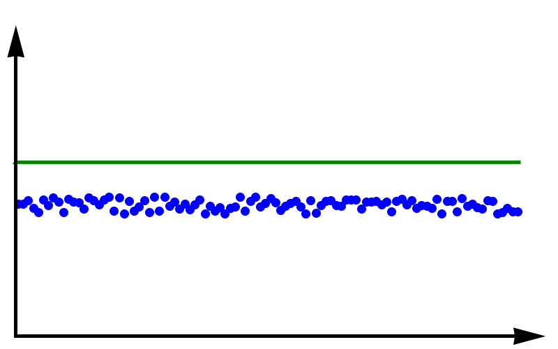
Data with high precision but low accuracy. The green line represents the true value.
A moral can be gained from this: just because you always get the same answer doesn’t mean the answer is correct.
When thinking about numerical methods you might object that calculations are deterministic. Therefore the outcome of repeating a calculation will always be the same. But there is a large class of algorithms that are not quite so deterministic. They might depend on an initial guess or even explicitly on some sequence of pseudo-random numbers. In these cases, repeating the calculation with a different guess or random sequence will lead to a different result.
What are Numbers? Or, Learning to Count!
Posted 17th April 2021 by Holger Schmitz
We all use numbers every day and some of us feel more comfortable dealing with them than others. But have you ever asked yourself what numbers really are? For example, what is the number 4? Of course, you can describe the symbol “4”. But that is not really the number, is it? You can use Roman numerals IV, Urdu ۴, or Chinese and Japanese Kanji 四. Each one of these symbols represents the same number. And yet, somehow we would all probably agree that there is only one number 4.
The question about the nature of numbers is twofold. You can understand this question purely mathematical one and ask for a clear definition of a number and the set of numbers in a mathematical sense. This will be the topic of this article. You can also ask yourself what numbers are in a philosophical sense. Do numbers exist? If yes, in what way do they exist, and what are they? This may be the topic of a future article.
Now that we have settled what type of question we want to answer, we should start with the simplest type of numbers. These are the natural numbers 0, 1, 2, 3, 4, …
I decided to include the number zero even though it might seem a little abstract at first. After all, what does it mean to have zero of something? But that objection strays into the philosophical realm again and, as I said above, I want to focus on the mathematical aspect here.
When doing the research for this article, I was slightly surprised at the plethora of different definitions for the natural numbers. But given how fundamental this question is, it should be no wonder that many mathematicians have thought about the problem of defining numbers and have come up with different answers.
The Peano Axioms
Let’s start with an axiomatic definition of numbers called the Peano axioms. This is one of the earliest strict definitions of the natural numbers in the modern sense. It doesn’t really state what the natural numbers are but focuses on how they behave. We start with the set of natural numbers, which we call $\mathbb{N}$, and a successor function $S$.
Peano Axiom 1:
$0$ is a natural number or, more formally, $0 \in \mathbb{N}$
This axiom just tells us that there is a natural number zero. We could have chosen 1 as the starting point but this is arbitrary.
Peano Axiom 2:
Every natural number $x$ has a successor $y$.
In other words, given that $x \in \mathbb{N}$ then it follows that $y = S(x) \in \mathbb{N}$.
Intuitively, the successor function will always produce the next natural number.
Mathematicians call this property of the natural number being closed under the successor operation $S$. All this means is that the successor operation will never produce a result that is outside of the natural numbers.
Peano Axiom 3:
If we have two natural numbers $x$ and $y$, and we know that the successors of $x$ and $y$ are equal, then this is the same as saying that $x$ and $y$ are equal.
Again, written more formally we say, given $x \in \mathbb{N}$ and $y \in \mathbb{N}$ and $S(x) = S(y)$ then it follows that $x=y$.
This means that any natural number cannot be the successor of two different number. In other words, if you have two different numbers then they can’t have the same successor.
Peano Axiom 4:
$0$ is not the successor of any other natural number.
In mathematical notation, if $x \in \mathbb{N}$ then $S(x) \ne 0$
At first sight, we might think that these axioms are complete. We can start from zero and use the successor function $S$ to iterate through the natural numbers. This is intuitively shown in the image below.
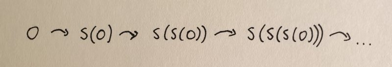
Repeatedly applying the successor function, starting from 0.
Here
1 = S(0)
2 = S(S(0)) = S(1)
3 = S(S(S(0))) = S(2)
and so on.
But we haven’t guaranteed that this iteration will eventually be able to reach all natural numbers. Imagine that, in addition to the above, there is some special number $z$ that creates a closed loop when applying the successor function. And this loop is separate from the sequence that we get when starting from zero.
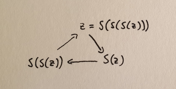
A closed loop of successors that isn’t connected to the zero element.
So we need another axiom that guarantees that all natural numbers are reachable from zero by repeatedly applying the successor function. This axiom is usually stated in the following way.
Peano Axiom 5: Axiom of Induction
Given any set $U \subseteq \mathbb{N}$ with $0 \in U$.
If $U$ is such that for every $n \in U$ the successor is also in $U$, i.e. $S(n) \in U$,
then $U = \mathbb{N}$
The idea behind this axiom is that $U$ can be chosen as the minimal set that contains no additional loops or numbers that are not reachable from zero. The fact that any set $U$ that contains zero and is closed under the successor function is identical to the natural numbers guarantees that all natural numbers are eventually reachable from zero. The axiom of induction is maybe more familiar in its alternative form.
Peano Axiom 5: Axiom of Induction, alternative form
Consider a mathematical statement that is true for zero.
If it can be proven that,
given the statement is true for a number $n$, then it is also true for $S(n)$,
then it follows that the statement is true for all natural numbers.
Here you can see that this axiom forms the basis of the familiar proof by induction.
Some Remarks
The Peano Axioms are helpful in defining the set of natural numbers $\mathbb{N}$ and arithmetic operations on them. But personally, I feel unsatisfied by this definition. The Peano Axioms tell us how natural numbers behave but they don’t really give any additional insight as to what numbers really are.
Take for example the number 2. We now know that 2 can be expressed as the successor of the successor of 0, i.e. $2 = S(S(0))$. We also know that this second successor must be a member of the set of natural numbers, but not much more. The problem here is that we never defined what the successor function should be.
Nonetheless, the Peano axioms can serve as a basis for more in-depth definitions of the natural numbers. These definitions can be considered models of the Peano Axioms in the sense that they define a zero element and some concrete successor function. The set of natural numbers can then be constructed from these and the Peano Axioms follow as consequences from these definitions.
In a future post, I will look at some set-theoretic definitions of the natural numbers. If you liked this post, please leave a comment and check back soon for more content.
The Euler Equations: Sod Shock Tube
Posted 30th September 2020 by Holger Schmitz
In the last post, I presented a simple derivation of the Euler fluid equations. These equations describe hydrodynamic flow in the form of three conservation equations. The three partial differential equations express the conservation of mass, the conservation of momentum, and the conservation of energy. These fundamental conservation equations are written in terms of fluxes of the densities of the conserved quantities.
In general, it is impossible to solve the Euler equations for an arbitrary problem. This means that in practice when we want to find the hydrodynamic flow in a particular situation, we have to use computers and numerical methods to calculate an approximation to the solution.
Numerical simulation codes approximate the continuous mathematical solution by storing the values of the functions at discrete points. The values are stored using a finite precision format. On most CPUs nowadays numbers will be stored as 64-bit floating-point, but for codes running on GPUs, this might be reduced to 32 bits. In addition to the discretisation in space, the equations are normally integrated using discrete steps in time. All of these factors mean that the computer only stores part of the information of the exact function.
These discretisations mean that the continuous differential equations have to be turned into a prescription how to update the discrete values from one time step to the next. For each differential equation, there are numerous ways to translate them into a numerical algorithm. Each algorithm will make different approximations and introduce different errors into the system. In general, it is impossible for a numerical algorithm to reproduce the solutions of the mathematical equations exactly. This will have implications for the physics that will be simulated with the code. Talking in terms of the Euler equations, some numerical algorithms will have problems capturing shocks, while others might smear out the solutions. Even others might cause the density to turn negative in places. Making sure that physical invariants, such as mass, momentum, and energy are conserved by the algorithm is often an important aspect when designing a numerical scheme.
The Sod Shock Tube
One of the standard tests for numerical schemes simulating the Euler equations is the Sod shock tube problem. This is a simple one-dimensional setup that is initialised with a single discontinuity in the density and energy density. It then develops a left-going rarefaction wave, a right-going shock and a somewhat slower right-going contact discontinuity. The shock tube has been proposed as a test for numerical schemes by Gary A. Sod 1978 [1]. It was then picked up by others like Philip Roe [2] or Bram van Leer [3] who made it popular. Now, it is one of the standard tests for any new solver for the Euler equations. The advantage of the Sod Shock Tube is that it has an analytical solution that can be compared against. I won’t go into the details of deriving the solution in this post. You can find a sketch of the procedure on Wikipedia.
Here, I want to present an example of the shock tube test using an algorithm by Kurganov, Noelle, and Petrova [4]. The advantage of the algorithm is that it is relatively easy to implement and that is straightforward to extend to multiple dimensions. I have implemented the algorithm in my open-source fluid code Vellamo. At the current stage, the code can only simulate the Euler equations, but it can run in 1d, 2d, or 3d. It is also parallelised so that it can run on computer clusters It uses the Schnek library to manage the computational grids, their distribution onto multiple CPUs, and the communication between the individual processes.
The video shows four simulations run with different grid resolutions. At the highest resolution of 10000 grid points, the results are more or less identical to the analytic solution. The left three panels show the density $\rho$, the momentum density $\rho v$, and the energy density $E$. These are the quantities that are actually simulated by the code. The right three panels show quantities derived from the simulation, the temperature $T$, the velocity $v$, and the pressure $p$.
Starting from the initial discontinuity at $x=0.5$ you can see a rarefaction wave moving to the left. The density $\rho$ has a negative slope whereas the momentum density $\rho v$ increases in this region. In the plot of the velocity, you can see a linear slope, indicating that the fluid is being accelerated by the pressure gradient. The expansion of the fluid causes cooling and the temperature $T$ decreases inside the rarefaction wave.
While the rarefaction wave moves left, a shock wave develops on the very right moving into the undisturbed fluid. All six graphs show a discontinuity at the shock. The density jumps $\rho$ as the fluid is compressed and the velocity $v$ rises from 0 to almost 1 as the expanding fluid pushes into the undisturbed background. The compression also causes a sudden increase in pressure $p$ and temperature $T$.
To the left of the shock wave, you can observe another discontinuity in some but not all quantities. This is what is known as a contact discontinuity. To the left of the discontinuity, the density $\rho$ is high and the temperature $T$ is low whereas to the right density $\rho$ is low and the temperature $T$ is high. Both effects cancel each other when calculating the pressure which is the same on both sides of the discontinuity. And because there is no pressure difference, the fluid is not accelerated either, and the velocity $v$ is the same on both sides as well.
If you look at the plots of the velocity $v$ and the pressure $p$ you can’t make out where the contact discontinuity is. In a way, this is quite extraordinary because these two quantities are calculated from the density $\rho$, the momentum density $\rho v$ and the energy density $E$. All of these quantities have jumps at the location of the contact discontinuity. The level to which the derived quantities stay constant across the discontinuity is an indicator of the quality of the numerical scheme.
The simulations with lower grid resolutions show how the scheme degrades. At 1000 grid points, the results are still very close to the exact solution. The discontinuities are slightly smeared out. If you look closely at the temperature profile, you can see a slight overshoot on the high-temperature side of the contact discontinuity. At 100 grid points, the discontinuities are more smeared out. The overshoot in the temperature is more pronounced and now you can also see an overshoot at the right end of the rarefaction wave. This overshoot is present in most quantities.
As a rule of thumb, a numerical scheme for hyperbolic differential equations has to balance accuracy against numerical diffusion. In regions where the solution is well behaved, high order schemes will provide very good accuracy. Near discontinuities, however, a high order scheme will tend to produce artificial oscillations. These artefacts can create non-physical behaviour when, for instance, the numerical solution predicts a negative density or temperature. A good scheme detects the conditions where the high order algorithm fails and falls back to a lower order in those regions. This will naturally introduce some numerical diffusion into the system.
At the lowest resolution with 50 grid points, the discontinuities are even more spread out. Nonetheless, at later times in the simulation, all discontinuities can be seen and the speed at which these discontinuities move compares well with the exact result.
I hope you have enjoyed this article. If you have any questions, suggestions, or corrections please leave a comment below. If you are interested in contributing to Vellamo or Schnek feel free to contact me via Facebook or LinkedIn.
[1] Sod, G.A., 1978. A survey of several finite difference methods for systems of nonlinear hyperbolic conservation laws. Journal of computational physics, 27(1), pp.1-31.
[2] Roe, P.L., 1981. Approximate Riemann solvers, parameter vectors, and difference schemes. Journal of computational physics, 43(2), pp.357-372.
[3] Van Leer, B., 1979. Towards the ultimate conservative difference scheme. V. A second-order sequel to Godunov’s method. Journal of Computational Physics, 32(1), pp.101-136.
[4] Kurganov, A., Noelle, S. and Petrova, G., 2001. Semidiscrete central-upwind schemes for hyperbolic conservation laws and Hamilton–Jacobi equations. SIAM Journal on Scientific Computing, 23(3), pp.707-740.
The Euler Equations
Posted 3rd September 2020 by Holger Schmitz
Leonhard Euler was not only brilliant but also a very productive mathematician. In this post, I want to talk about one of the many things named after the Swiss genius, the Euler equations. These should not be confused with the Euler identity, that famous relation involving $e$, $i$, and $\pi$. No, the Euler equations are a set of partial differential equations that can be used to describe fluid flow. They are related to the Navier-Stokes equations which are at the heart of one of the unsolved Millenium Problems of the Clay Mathematics Institute.
In this short series of posts, I want to present a phenomenological derivation of the equations in one dimension. This derivation is not mathematically rigorous, but will hopefully give you an understanding of the physics that the equations are describing.
Conservation Laws
One way to understand the Euler equations is to write them in the form of conservation laws. Each equation represents a basic conservation law of physics. A central concept in these conservation equation is flux. In a 1d description, the flux of a quantity is a measure for the amount of that quantity that passes through a point. In 2d it’s the amount passing through a line and in 3d through a surface, but let’s stick to 1d during this article.
Take some quantity $N$. To make it concrete, imagine something like the total mass or number of atoms in a volume. I am using the word volume loosely. In 1d a volume is the same as an interval. Let’s call the flux of this quantity $F$. The flux can be different at different locations, so $F$ is a function of position $x$, in other words, the flux is $F(x)$.
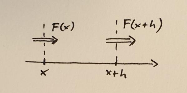
Flux into and out of a small volume between $x$ and $x+h$
Next, consider a small volume between $x$ and $x+h$. Here $h$ is the width of the volume and you should think of it as a small quantity. The rate of change of the quantity $N$ within this volume is determined by the difference between the flux into the volume and the flux out of the volume. If we take positive flux to mean that the quantity (mass, number of atoms, stuff) is moving to the right, then we can write down the following equation.
$$\frac{dN}{dt} = F(x) – F(x+h)$$
Here the left-hand side of the equation represents the rate of change of $N$. I have not written it here but, of course, $N$ depends on the position $x$ as well as the with of the volume $h$. The next step to turn this into a conservation equation is to divide both sides by $h$.
$$\frac{d}{dt}\left(\frac{N}{h}\right) = -\frac{F(x+h) – F(x)}{h}$$
If you remember your calculus lessons, you might already see where this is going. We now make $h$ smaller and smaller and look at the limit when $h \to 0$. The right hand side of the equation will give us the derivative of $F$,
$$\lim_{h \to 0} \frac{F(x+h) – F(x)}{h} = \frac{dF}{dx}$$
The amount of stuff $N$ in the volume will shrink and shrink as $h$ decreases, but because we are dividing by $h$ the ratio $N/h$ will converge to a sensible value. Let’s call this value $n$,
$$n = \lim_{h \to 0}\frac{N}{h}.$$
The quantity $n$ is called the density of $N$. Now the conservation law is simply written as
$$\frac{\partial n}{\partial t} = -\frac{\partial F}{\partial x}.$$
This equation expresses the change of the density of the conserved quantity through the derivative of the flux of that quantity.
The Equations
Now that the basic form of the conservation equations is established, let’s look at some quantities that are conserved and that can be used to express fluid flow. The first conservation law to look at is the conservation of mass. Note again that the conservation equation is written in terms of the density of the conserved quantity. The mass density is the mass contained in a small volume divided by that volume. It is often abbreviated by the Greek letter $\rho$ (rho).
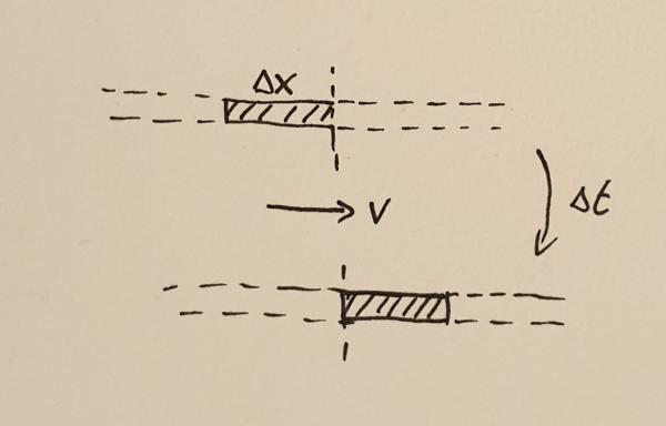
Matter crossing a point during the time interval $\Delta t$
In order to find out what the mass flux is, consider the fluid moving with velocity $v$ through some point. During a small time interval, $\Delta t$ the fluid will move by a small distance $\Delta x$. All the mass $M$ contained in the interval of width $\Delta x$ will cross the point. This mass can be calculated to be
$$M = \rho \Delta x.$$
The flux is the amount of mass crossing the point divided by the time it took the mass to cross that point, $F_{\rho} = M / \Delta t$. In other words,
$$F_{\rho} = \rho \frac{\Delta x}{\Delta t} = \rho v.$$
This now lets us write the mass conservation equation,
$$\frac{\partial \rho}{\partial t} = -\frac{\partial }{\partial x}(\rho v).$$
What does this equation mean? Let me explain this with two examples. First, imagine a constant flow velocity $v$ but an increasing density profile $\rho(x)$. At any given point the density will decrease because the density profile will constantly move towards the right without changing shape. The lower density that was previously located at somewhat left of $x$ will move to the point $x$ thus decreasing the density there.
For the other example, imagine that the density is constant but the velocity has an increasing profile. Matter to the right will flow faster than matter to the left. This will also decrease the density over time because the existing mass is constantly thinned out.
The next conservation equation expresses the conservation of momentum. Momentum is mass times velocity and therefore momentum density is mass density times velocity, $\rho v$. In the mass conservation equation, you could see that the flux consists only of the conserved density multiplied with the velocity. This is called the convective term and this term is present in all Euler equations. However, the momentum can also change through a force. Without external forces, the only force onto each fluid element is through the pressure $p$. The momentum conservation equation can be written as
$$\frac{\partial }{\partial t}(\rho v) = -\frac{\partial }{\partial x}(\rho v^2 + p).$$
The last conservation equation is the conservation of energy, expressed by the energy density $e$,
$$\frac{\partial e}{\partial t} = -\frac{\partial }{\partial x}(e v + p v).$$
The first term is again the convective term expressing the transport of energy contained in the fluid as the fluid moves. The second term is the work done by the pressure force. Note that the energy density $e$ contains the internal (heat) energy as well as the kinetic energy of the fluid moving as a whole.
Finally, we need to close the set of equations by defining what the pressure $p$ is. This closure depends on the type of fluid you want to model. For an ideal gas, the pressure is related to the other variables through
$$p = (\gamma – 1)\left(E – \frac{\rho v^2}{2}\right).$$
Here $\gamma$ is the adiabatic gas index. The second bracket on the right-hand side is the internal energy, expressed as the total energy minus the kinetic energy of the flow.
Putting it All Together
In summary, the Euler equations are conservation equations for the mass, momentum, and energy in the system. In 1d, they can be written as
$$\begin{eqnarray}
\frac{\partial }{\partial t}\rho &=& -\frac{\partial }{\partial x}(\rho v) \\
\frac{\partial }{\partial t}(\rho v) &=& -\frac{\partial }{\partial x}(\rho v^2 + p) \\
\frac{\partial }{\partial t}e &=& -\frac{\partial }{\partial x}(e v + p v)
\end{eqnarray}
$$
In higher dimensions, the derivative with respect to $x$ is replaced by the divergence operator $\nabla$.
$$\begin{eqnarray}
\frac{\partial }{\partial t}\rho &=& -\nabla(\rho \mathbf{v}) \\
\frac{\partial }{\partial t}(\rho v) &=& -\nabla(\rho \mathbf{v}\otimes\mathbf{v} + p\mathbf{I}) \\
\frac{\partial }{\partial t}e &=& -\nabla(e \mathbf{v} + p \mathbf{v})
\end{eqnarray}
$$
The $\otimes$ symbol denotes the outer product of the velocity vectors. It multiplies two vectors to produce a matrix. I will not go into the definition of the outer product here. You can read more on Wikipedia. The symbol $\mathbf{I}$ is the identity matrix.
Summary
The Euler equations are a set of partial differential equations describing fluid flow. When Euler published a simpler version of these equations, they were one of the earliest examples of partial differential equations. Today, the Euler equations and their generalisations, including the Navier-Stokes equations provide the basis for understanding fluid behaviour, turbulence, and the weather.
The Euler equations are difficult to solve and only some special solutions can be written down on paper. For the general case, we need computers to give us answers. In the next post, I will show the results of some simulations I have created with my freely available fluid code Vellamo.
Computational Physics Basics: Integers in C++, Python, and JavaScript
Posted 5th August 2020 by Holger Schmitz
In a previous post, I wrote about the way that the computer stores and processes integers. This description referred to the basic architecture of the processor. In this post, I want to talk about how different programming languages present integers to the developer. Programming languages add a layer of abstraction and in different languages that abstraction may be less or more pronounced. The languages I will be considering here are C++, Python, and JavaScript.
Integers in C++
C++ is a language that is very close to the machine architecture compared to other, more modern languages. The data that C++ operates on is stored in the machine’s memory and C++ has direct access to this memory. This means that the C++ integer types are exact representations of the integer types determined by the processor architecture.
The following integer datatypes exist in C++
| Type | Alternative Names | Number of Bits | G++ on Intel 64 bit (default) |
|---|---|---|---|
char |
at least 8 | 8 | |
short int |
short |
at least 16 | 16 |
int |
at least 16 | 32 | |
long int |
long |
at least 32 | 64 |
long long int |
long long |
at least 64 | 64 |
This table does not give the exact size of the datatypes because the C++ standard does not specify the sizes but only lower limits. It is also required that the larger types must not use fewer bits than the smaller types. The exact number of bits used is up to the compiler and may also be changed by compiler options. To find out more about the regular integer types you can look at this reference page.
The reason for not specifying exact sizes for datatypes is the fact that C++ code will be compiled down to machine code. If you compile your code on a 16 bit processor the plain int type will naturally be limited to 16 bits. On a 64 bit processor on the other hand, it would not make sense to have this limitation.
Each of these datatypes is signed by default. It is possible to add the signed qualifier before the type name to make it clear that a signed type is being used. The unsigned qualifier creates an unsigned variant of any of the types. Here are some examples of variable declarations.
char c; // typically 8 bit
unsigned int i = 42; // an unsigned integer initialised to 42
signed long l; // the same as "long l" or "long int l"
As stated above, the C++ standard does not specify the exact size of the integer types. This can cause bugs when developing code that should be run on different architectures or compiled with different compilers. To overcome these problems, the C++ standard library defines a number of integer types that have a guaranteed size. The table below gives an overview of these types.
| Signed Type | Unsigned Type | Number of Bits |
|---|---|---|
int8_t |
uint8_t |
8 |
int16_t |
uint16_t |
16 |
int32_t |
uint32_t |
32 |
int64_t |
uint64_t |
64 |
More details on these and similar types can be found here.
The code below prints a 64 bit int64_t using the binary notation. As the name suggests, the bitset class interprets the memory of the data passed to it as a bitset. The bitset can be written into an output stream and will show up as binary data.
#include  <bitset>

void printBinaryLong(int64_t num) {
    std::cout << std::bitset<64>(num) << std::endl;
}
Integers in Python
Unlike C++, Python hides the underlying architecture of the machine. In order to discuss integers in Python, we first have to make clear which version of Python we are talking about. Python 2 and Python 3 handle integers in a different way. The Python interpreter itself is written in C which can be regarded in many ways as a subset of C++. In Python 2, the integer type was a direct reflection of the long int type in C. This meant that integers could be either 32 or 64 bit, depending on which machine a program was running on.
This machine dependence was considered bad design and was replaced be a more machine independent datatype in Python 3. Python 3 integers are quite complex data structures that allow storage of arbitrary size numbers but also contain optimizations for smaller numbers.
It is not strictly necessary to understand how Python 3 integers are stored internally to work with Python but in some cases it can be useful to have knowledge about the underlying complexities that are involved. For a small range of integers, ranging from -5 to 256, integer objects are pre-allocated. This means that, an assignment such as
n = 25
will not create the number 25 in memory. Instead, the variable n is made to reference a pre-allocated piece of memory that already contained the number 25. Consider now a statement that might appear at some other place in the program.
a = 12
b = a + 13
The value of b is clearly 25 but this number is not stored separately. After these lines b will reference the exact same memory address that n was referencing earlier. For numbers outside this range, Python 3 will allocate memory for each integer variable separately.
Larger integers are stored in arbitrary length arrays of the C int type. This type can be either 16 or 32 bits long but Python only uses either 15 or 30 bits of each of these "digits". In the following, 32 bit ints are assumed but everything can be easily translated to 16 bit.
Numbers between −(230 − 1) and 230 − 1 are stored in a single int. Negative numbers are not stored as two’s complement. Instead the sign of the number is stored separately. All mathematical operations on numbers in this range can be carried out in the same way as on regular machine integers. For larger numbers, multiple 30 bit digits are needed. Mathamatical operations on these large integers operate digit by digit. In this case, the unused bits in each digit come in handy as carry values.
Integers in JavaScript
Compared to most other high level languages JavaScript stands out in how it deals with integers. At a low level, JavaScript does not store integers at all. Instead, it stores all numbers in floating point format. I will discuss the details of the floating point format in a future post. When using a number in an integer context, JavaScript allows exact integer representation of a number up to 53 bit integer. Any integer larger than 53 bits will suffer from rounding errors because of its internal representation.
const a = 25;
const b = a / 2;
In this example, a will have a value of 25. Unlike C++, JavaScript does not perform integer divisions. This means the value stored in b will be 12.5.
JavaScript allows bitwise operations only on 32 bit integers. When a bitwise operation is performed on a number JavaScript first converts the floating point number to a 32 bit signed integer using two’s complement. The result of the operation is subsequently converted back to a floating point format before being stored.
Computational Physics Basics: How Integers are Stored
Posted 4th April 2020 by Holger Schmitz
Unsigned Integers
Computers use binary representations to store various types of data. In the context of computational physics, it is important to understand how numerical values are stored. To start, let’s take a look at non-negative integer numbers. These unsigned integers can simply be translated into their binary representation. The binary number-format is similar to the all-familiar decimal format with the main difference that there are only two values for the digits, not ten. The two values are 0 and 1. Numbers are written in the same way as decimal numbers only that the place values of each digit are now powers of 2. For example, the following 4-digit numbers show the values of the first four

0 0 0 1 decimal value 20 = 1
0 0 1 0 decimal value 21 = 2
0 1 0 0 decimal value 22 = 4
1 0 0 0 decimal value 23 = 8
The binary digits are called bits and in modern computers, the bits are grouped in units of 8. Each unit of 8 bits is called a byte and can contain values between 0 and 28 − 1 = 255. Of course, 255 is not a very large number and for most applications, larger numbers are needed. Most modern computer architectures support integers with 32 bits and 64 bits. Unsigned 32-bit integers range from 0 to 232 − 1 = 4, 294, 967, 295 ≈ 4.3 × 10⁹ and unsigned 64-bit integers range from 0 to 264 − 1 = 18, 446, 744, 073, 709, 551, 615 ≈ 1.8 × 10¹⁹. It is worthwhile noting that many GPU architectures currently don’t natively support 64-bit numbers.
The computer’s processor contains registers that can store binary numbers. Thus a 64-bit processor contains 64-bit registers and has machine instructions that perform numerical operations on those registers. As an example, consider the addition operation. In binary, two numbers are added in much the same way as using long addition in decimal. Consider the addition of two 64 bit integers 7013356221863432502 + 884350303838366524. In binary, this is written as follows.
  01100001,01010100,01110010,01010011,01001111,01110010,00010001,00110110
+ 00001100,01000101,11010111,11101010,01110101,01001011,01101011,00111100
---------------------------------------------------------------------------
  01101101,10011010,01001010,00111101,11000100,10111101,01111100,01110010
The process of adding two numbers is simple. From right to left, the digits of the two numbers are added. If the result is two or more, there will be a carry-over which is added to the next digit on the left.
You could add integers of any size using this prescription but, of course, in the computer numbers are limited by the number of bits they contain. Consider the following binary addition of (264 − 1) and 1 .
  11111111,11111111,11111111,11111111,11111111,11111111,11111111,11111111
+ 00000000,00000000,00000000,00000000,00000000,00000000,00000000,00000001
---------------------------------------------------------------------------
  00000000,00000000,00000000,00000000,00000000,00000000,00000000,00000000
If you were dealing with mathematical integers, you would expect to see an extra digit 1 on the left. The computer cannot store that bit in the register containing the result but stores the extra bit in a special carry flag. In many computer languages, this unintentional overflow will go undetected and the programmer has to take care that numerical operations do not lead to unintended results.
Signed Integers
The example above shows that adding two non-zero numbers can result in 0. This can be exploited to define negative numbers. In general, given a number a, the negative − a is defined as the number that solves the equation
a + ( − a) = 0.
Mathematically, the N-bit integers can be seen as the group of integers modulo 2N. This means that for any number a ∈ {0, …, 2N − 1} the number − a can be defined as
− a = 2N − a ∈ {0, …, 2N − 1}.
By convention, all numbers whose highest value binary bit is zero are considered positive. Those numbers whose highest value bit is one are considered negative. This makes the addition and subtraction of signed integers straightforward as the processor does not need to implement different algorithms for positive or negative numbers. Signed 32-bit integers range from − 2, 147, 483, 648 to 2, 147, 483, 647, and 64-bit integers range from − 9, 223, 372, 036, 854, 775, 808 to 9, 223, 372, 036, 854, 775, 807.
This format of storing negative numbers is called the two’s complement format. The reason for this name becomes obvious when observing how to transform a positive number to its negative.
01100001,01010100,01110010,01010011,01001111,01110010,00010001,00110110 (7013356221863432502)
10011110,10101011,10001101,10101100,10110000,10001101,11101110,11001010 (-7013356221863432502)
To invert a number, first, invert all its bits and then add 1. This simple rule of taking the two’s complement can be easily implemented in the processor’s hardware. Because of the simplicity of this prescription, and the fact that adding a negative number follows the same algorithm as adding a positive number, two’s complement is de-facto the only format used to store negative integers on modern processors.
Exercises
- Show that taking the two’s complement of an N-bit number a does indeed result in the negative − a if the addition of two numbers is defined as the addition modulo 2N.
- Find out how integers are represented in the programming language of your choice. Does this directly reflect the representation of the underlying architecture? I will be writing another post about this topic soon.
- Most processors have native commands for multiplying two integers. The result of multiplying the numbers in two N-bit registers are stored in two N-bit result registers representing the high and low bits of the result. Show that the resulting 2N bits will always be enough to store the result.
- Show how the multiplication of two numbers can be implemented using only the bit-shift operator and conditional addition based on the bit that has been shifted out of the register. The bit-shift operator simply shifts all bits of a register to the left or right.
String Art and Heart Curves
Posted 12th March 2020 by Holger Schmitz
In my childhood, my parents would take us to the seaside for the summer holidays. One thing, other than the sun and the beach, that I distinctly remember were the nautic decorations in the cafes. One particular image was an abstract picture of a sailboat made from some nails hammered into a wooden board and pieces of string that were tied around those nails. It always fascinated me, how this simple arrangement of straight lines could create such a beautiful and dynamic image. Around the same time, in primary school, we used a similar technique in art class, with needle and thread and a piece of cardboard, to create an image of a snowflake.
It wasn’t until much later that I understood that the curves created by the thread could be described using mathematics. But while I knew that this had to do with maths somehow, during my school years I always thought that the maths was much too complicated for me to understand. Now, I have children and they have been doing similar art projects. From a teaching perspective, I am aware that these projects are intended to create an interest in maths. I think there is a missed opportunity when these line patterns are only used in primary school art lessons. The mathematics of the curves created by these lines can be accessible to secondary school students.
As an example, I want to present here the curve created by drawing straight lines in a circle. Here is the recipe:
- Draw a large circle on a piece of paper
- Draw a reasonably large number of equally spaced points around the circumference, about 20 to 30 should be OK
- Choose a point as point 0 and number the points around the circle, clockwise or anticlockwise
- Now draw a line
- from point 1 to point 2
- from point 2 to point 4
- from point 3 to point 6
- and so on, always connecting point $n$ with point $2n$.
Once the starting point has reached the opposite side, the endpoint will have reached point 0. Keep going by always incrementing the endpoint by two while moving the starting point by one.
You should end up with something like this.
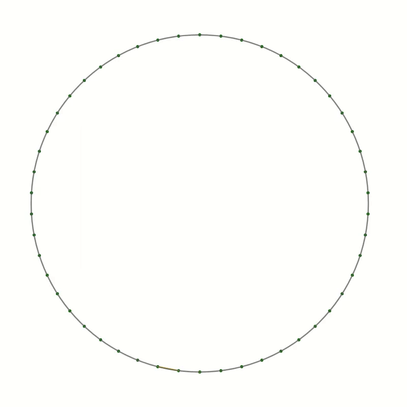
As you can see the lines you have drawn create an interesting pattern. In fact, the lines trace out a curve called the cardioid or heart curve. Each line you have drawn is a tangent to the cardioid. This means that each of the lines touches the cardioid in a single point.
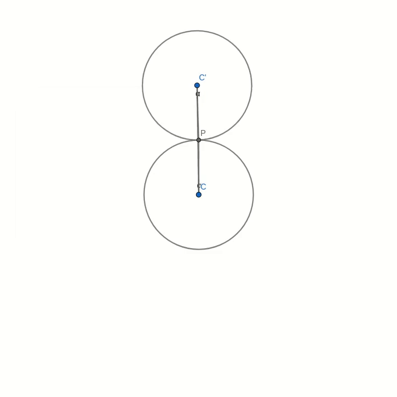
Let’s take a look at this cardioid curve. It is a special case of an epicycloid. This family of curves is generated by tracing a point on the circumference of one circle as it rolls around another circle. In the case of the cardioid, both circles have the same radius. The point that traces the curve is chosen to lie on the circumference of the outer circle. In the picture below you can see how the cardioid is created.
The curves in the two pictures look similar and if you were to place one image on top of the other, you would not see any difference in the curves. That seems to suggest that the two are in fact identical. But comparing images is not a mathematical proof. And surely you don’t believe this statement just because everybody on the internet claims it to be true.
If you look around, you can find several proofs that show you that the curve created by our string art is indeed the cardioid. But most of these proofs make use of trigonometry. This makes them inaccessible to anybody who is not yet comfortable with trigonometric identities. I believe that a purely geometric proof is easier to understand and also more beautiful than resorting to sine and cosine functions.
The proof
I order to prove the identity of the two curves we need to show two things. First, we need to show that our line construction intersects the cardioid in at least one point and we need to find that point. Then we need to show that the point that traces the cardioid moves in the direction of the line segment. This second part of the proof shows that the line segments are tangential to the cardioid.
Part 1: Constructing a point on the cardioid
Look at the figure below. Don’t get too confused with all the lines and angles in the picture. I will explain everything bit by bit. Remember when you were drawing the string art picture. You were drawing a line from some start point to some endpoint. In the diagram below, I have taken one of those lines and named the start point B and the endpoint B’. I have also connected the origin point 0 to the start point B. Now, B’ moves around the circle twice as fast as point B. This means that the distance from B to B’ is the same as the distance from 0 to B. In other words, if you draw a line from the centre C of the big circle to B, the figure is symmetric with respect to that line.
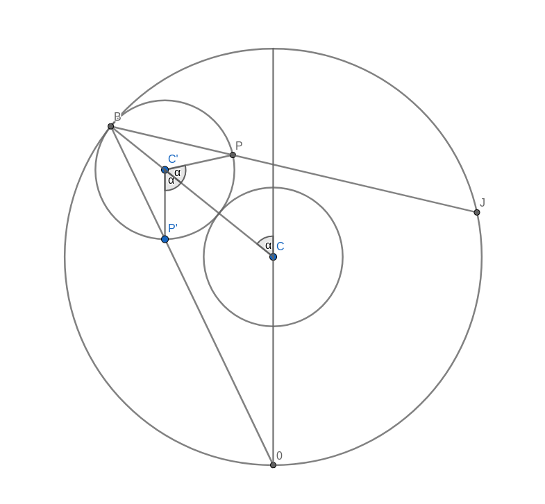
Now, look at the two small circles. The circle at the centre C of the large circle stays fixed. The small circle centred at C’ on the connection between C and B is the circle that rolls along the circumference and creates the cardioid. The line B-B’ intersects this outer circle at a point P. We need to show that this intersection point P is the same as the point that stays fixed on the outer circle as it rolls along. We can prove this by showing that the angle C-C’-P is the same as the angle that C-C’ makes with the vertical through the central point C.
Take the intersection between the line A-B and the rolling circle and call it P’. You can immediately see that the triangles A-B-C and P’-B-C’ are similar. This means that the line P’-C’ is vertical, just like the line A-C. It follows that the angle C-C’-P’ is the same as the angle that C-C’ makes with the vertical because they are opposite angles. But because of the symmetry of the construction, this angle is also the same as C-C’-P.
With this, we have shown that the intersection point P is, in fact, a point on the cardioid curve.
Part 2: Direction of motion of P
The motion of the point P, as the outer small circle rolls around the inner circle, is made up of two contributions. The first is the motion of the centre C’ orbiting around the inner circle. The second is the motion due to the rolling circle spinning around its own centre. We need to look at the direction and magnitude of each of these velocities.
Let’s say that the radius of the small circles is 1 and the angular velocity of the rotation of the outer circle around the inner is also 1. The exact values are not important because we only need to compare the two contributions of the velocity of point P. We don’t need to find its absolute value.
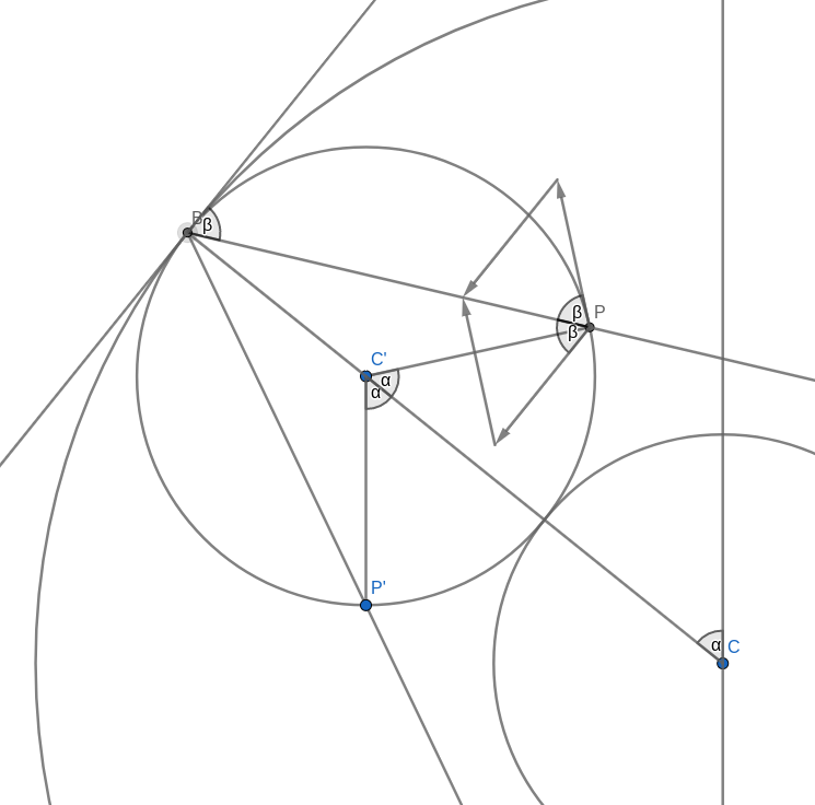
Orbital Velocity
The orbital velocity is oriented perpendicular to the connection C-B which also is parallel to the tangent to the circle through B. This means that naturally, the angle between this velocity and the line B-P is the same as the angle between the tangent and B-P. To compare the magnitudes we have to remember some equation from physics. The speed of a point rotating around a centre is the product of the distance to the centre and the angular velocity. Let’s call the radius of the small circle $R$ and the angular velocity of the rotation of the outer circle around the inner circle $\omega$ (that’s the lowercase Greek letter omega). The distance of the outer centre to the centre of rotation is $2R$ and this makes the speed of the orbital rotation equal to
$$v_{\text{orbit}} = 2R\omega.$$
Now let’s look at the velocity of the spin rotation. The point P rotates around the centre of rotation C’. The radius is $R$ but the angular velocity is $2\omega$. To see this, look at the vertical line C’-P’. This line stays vertical at all times. In part 1 of the proof we already saw that that the angle C-C’-P’ is the same as the angle that C-C’ makes with the vertical, so as C’ moves around C by some angle, C-C’-P’ will increase by the same amount. But so will C-C’-P. This means that the angle P’-C-P increases twice as fast as the orbital angle. The resulting speed of the spin motion is
$$v_{\text{spin}} = R\times 2\omega.$$
We can see that the magnitude of the velocity of the spin motion is equal to that of the orbital motion. We also saw that the line B-P halves the angle between those two velocities. This means that the sum of these two velocities must lie in the direction of B-P. In other words, B-P is a tangent to the motion of the point P which is what we needed to prove.
Summary
I admit that this proof is somewhat lengthy but I do think that it gives some interesting insight into why the pattern of lines created by our initial construction generates the cardioid curve. All the figures for this post were created with Geogebra and are available online.